Y-Intercept

In a simple regression model, the y-intercept is the expected value of the dependent variable when the independent variable equals zero. In the regression equation Y = a + bX, a is the y-intercept. Visually, in a two-dimensional scatter plot with a regression line, the y-intercept is the value of y where the regression line crosses the vertical axis. In a multiple regression model, the intercept is the expected value of the dependent variable when all independent variables equal zero.

Consider the following example, in which a researcher is interested in factors that reduce heart disease, or at least reduce the most harmful effects of heart disease. In particular, this researcher wants to examine the relationship between wine consumption (X variable) and deaths from heart disease (Y variable). The main hypothesis is that increased wine consumption may lower the risks of heart disease. The researcher gathers data on annual wine consumption (liters per person) and heart disease deaths (per 100,000 population) from several countries. The estimated regression model from the data is Y = 261 – 23X. In this example, the y-intercept is 261, indicating that in a hypothetical country with no wine consumption, the model predicts 261 deaths from heart disease for every 100,000 people in the country. The data are plotted in Figure 1 below, with the regression line included. The value of the y-intercept is noted in the figure.

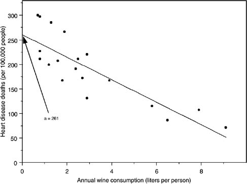
Figure 1 Scatterplot With y-Intercept Identified

Moore (1998), p. 314.

Because Y = a when X = 0, the y-intercept is also called the “constant” in the regression equation. In some substantive situations, the researcher may decide for theoretical reasons that the dependent variable should always be zero when the independent variable is zero. In that case, the regression equation can be calculated with no constant (so that a is zero), and the simple [Page 1202]regression equation becomes Y = bX. Graphically, this would correspond to a regression line through the origin.