
Entry
Reader's guide
Entries A-Z
X¯ is the notation for the arithmetic Mean of a Variable. If the variable is denoted by X, the ith observation’s value on variable X is denoted by Xi, and N is the total number of observations, then X¯ = ∑ Xi/N. Figure 1 shows a density plot of spending on elementary and secondary education in the 50 American states, with the mean indicated on the graph.
The mean is most appropriate as a measure of central tendency when the data are numeric, though the median might be more appropriate when there are outliers on the variable. The mean also can be computed for dichotomous variables (scored as either “1” or “0”), in which case the mean is simply the proportion of cases in the “1” category. The mean is also often computed for ordinal measures, though that use is debatable. For example, Gravetter and Wallnau (2000) argued against calculating the mean and other traditional statistics with ordinal variables because the distance between values, and hence the mean, is not well defined. However, Borgatta and Bohrnstedt (1980) instead argued that there are latent continuous variables underlying ordinal variables, so results obtained with integer scoring would be fairly close to those that would be obtained for the true unknown numbered categories.
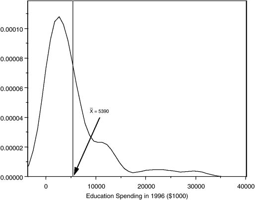
Figure 1 Density Plot With Mean Identified
X¯ has several distinctive properties leading to interpretations of the mean. First, the sum of signed deviations around the mean is zero. That is ∑(Xi − X¯) = 0. Furthermore, the sum of signed deviations around any value other than the mean is larger. As a result, the mean is considered a “best guess” statistic, in that guessing that the value of an observation is the mean leads to a smaller total error than would any other guess.
Second, the sum of positive deviations from the mean equals the sum of negative deviations from the mean (which is why the sum of signed deviations around the mean is zero). Becauseof that property, the mean is sometimes described as the fulcrum (or balance point) of the variable’s distribution. To the extent that some values are above X¯, they are balanced off by other values below X¯.
Third, the sum of squared deviations around X¯ is smaller than the sum of squared deviations around any over value. This leastsquares property of the mean is why variances are computed around the mean.
Additionally, X¯ is a consistent, unbiased, and efficient estimator of the variable's Population mean. It is consistent because the probability that X¯ minus the population mean is less than any value (δ) approaches 1 as the number of observations becomes infinitely large. It is unbiased because its expectation is the population mean. X¯ is considered efficient because the variance of Sample means around their mean is smaller than it would be for any other estimator of the population mean.
References
...
- Analysis of Variance
- Association and Correlation
- Association
- Association Model
- Asymmetric Measures
- Biserial Correlation
- Canonical Correlation Analysis
- Correlation
- Correspondence Analysis
- Intraclass Correlation
- Multiple Correlation
- Part Correlation
- Partial Correlation
- Pearson's Correlation Coefficient
- Semipartial Correlation
- Simple Correlation (Regression)
- Spearman Correlation Coefficient
- Strength of Association
- Symmetric Measures
- Basic Qualitative Research
- Basic Statistics
- F Ratio
- N(n)
- t-Test
- X¯
- Y Variable
- z-Test
- Alternative Hypothesis
- Average
- Bar Graph
- Bell-Shaped Curve
- Bimodal
- Case
- Causal Modeling
- Cell
- Covariance
- Cumulative Frequency Polygon
- Data
- Dependent Variable
- Dispersion
- Exploratory Data Analysis
- Frequency Distribution
- Histogram
- Hypothesis
- Independent Variable
- Measures of Central Tendency
- Median
- Null Hypothesis
- Pie Chart
- Regression
- Standard Deviation
- Statistic
- Causal Modeling
- DISCOURSE/CONVERSATION ANALYSIS
- Econometrics
- Epistemology
- Ethnography
- Evaluation
- Event History Analysis
- Experimental Design
- Factor Analysis and Related Techniques
- Feminist Methodology
- Generalized Linear Models
- HISTORICAL/COMPARATIVE
- Interviewing in Qualitative Research
- Latent Variable Model
- LIFE HISTORY/BIOGRAPHY
- LOG-LINEAR MODELS (CATEGORICAL DEPENDENT VARIABLES)
- Longitudinal Analysis
- Mathematics and Formal Models
- Measurement Level
- Measurement Testing and Classification
- Multilevel Analysis
- Multiple Regression
- Qualitative Data Analysis
- Sampling in Qualitative Research
- Sampling in Surveys
- Scaling
- Significance Testing
- Simple Regression
- Survey Design
- Time Series
- ARIMA
- Box-Jenkins Modeling
- Cointegration
- Detrending
- Durbin-Watson Statistic
- Error Correction Models
- Forecasting
- Granger Causality
- Interrupted Time-Series Design
- Intervention Analysis
- Lag Structure
- Moving Average
- Periodicity
- Serial Correlation
- Spectral Analysis
- Time-Series Cross-Section (TSCS) Models
- Time-Series Data (Analysis/Design)
- Trend Analysis
Get a 30 day FREE TRIAL
-
 Watch videos from a variety of sources bringing classroom topics to life
 -
Read modern, diverse business cases
-
Explore hundreds of books and reference titles

Read next

More like this
Sage Recommends
We found other relevant content for you on other Sage platforms.
Have you created a personal profile? Login or create a profile so that you can save clips, playlists and searches