
Entry
Reader's guide
Entries A-Z
Spectral Analysis
Spectral analysis is one method of identifying the cyclical components of time-series data. Cycles are periodic events typically represented as a waveform of the trigonometric sine or cosine function, or sinusoid, represented graphically and mathematically by Figure 1:
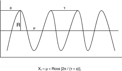
Figure 1 Spectral Analysis
where τ represents the period of the waveform, or the distance from one peak of the cycle to another; μ represents the mean of the highest and lowest points of the waveform; φ represents the initial phase of the wave; and R represents the amplitude, or distance from peak to trough, of the waveform.
The sinusoid is an important component of cyclical analysis because it is used to model the shape of those cycles. Where complex waveforms exist, researchers and statistical packages may model the cycles using several sinusoidal components. Although it is still possible to model the data if cycles deviate substantially from the sinusoid, such methods are mathematically complex and less tractable than the model presented here.
The cyclical nature of time-series data can be approximated once time trends are removed from the data by partitioning the residual variance in a time-series that is not due to a linear or curvilinear trend in the data. The total sum of squares is divided into a set of N/2 sum of squares components, each with 2 degrees of freedom. The estimates derived from the calculations are transformed into the sum of squares accounted for by each periodic component, to create intensity estimates.
In order to shrink the wide confidence intervals often associated with intensity estimates, spectral analysis smoothes the estimates to create a power spectrum. Smoothing procedures compute weighted averages of intensity estimates within a few neighboring frequencies. Variations in the number of neighboring frequencies (or width) included in the weighted average and variations in the weights applied, resulting from the use of different smoothing techniques, can produce more reliable estimates of the cyclical nature of the data. For instance, Daniell (equal weight) smoothing techniques with a width (or M) of 3 replace the intensity estimates for frequency i, with the mean for three ordinates, including i − 1, i, and i + 1. Equal weights (or 1/M) are applied to the new estimates, (1/3)× intensity at frequency (i−1)+(1/3)× intensity at frequency i + (1/3)× intensity at frequency (i + 1), to achieve a smoothed estimate of cycles. It is worth noting that the size of confidence intervals decreases as the number of neighboring frequencies increases. However, excessive smoothing can distort the data and make it difficult to make clear judgments about the lengths of cycles in the data (or τ).
Once the power spectrum is calculated, it is divided by the total amount of power or variance, producing a spectral density function. The results are typically plotted with the spectral density on the y-axis and the frequency (1/τ) on the x-axis. Data that exhibit a 4-year cycle would register a frequency of 1/4 or .25 at its peak, which would be visible on a smoothed graph. Statistical significance is determined through the estimation of confidence intervals based on chi-square
...
- Analysis of Variance
- Association and Correlation
- Association
- Association Model
- Asymmetric Measures
- Biserial Correlation
- Canonical Correlation Analysis
- Correlation
- Correspondence Analysis
- Intraclass Correlation
- Multiple Correlation
- Part Correlation
- Partial Correlation
- Pearson's Correlation Coefficient
- Semipartial Correlation
- Simple Correlation (Regression)
- Spearman Correlation Coefficient
- Strength of Association
- Symmetric Measures
- Basic Qualitative Research
- Basic Statistics
- F Ratio
- N(n)
- t-Test
- X¯
- Y Variable
- z-Test
- Alternative Hypothesis
- Average
- Bar Graph
- Bell-Shaped Curve
- Bimodal
- Case
- Causal Modeling
- Cell
- Covariance
- Cumulative Frequency Polygon
- Data
- Dependent Variable
- Dispersion
- Exploratory Data Analysis
- Frequency Distribution
- Histogram
- Hypothesis
- Independent Variable
- Measures of Central Tendency
- Median
- Null Hypothesis
- Pie Chart
- Regression
- Standard Deviation
- Statistic
- Causal Modeling
- DISCOURSE/CONVERSATION ANALYSIS
- Econometrics
- Epistemology
- Ethnography
- Evaluation
- Event History Analysis
- Experimental Design
- Factor Analysis and Related Techniques
- Feminist Methodology
- Generalized Linear Models
- HISTORICAL/COMPARATIVE
- Interviewing in Qualitative Research
- Latent Variable Model
- LIFE HISTORY/BIOGRAPHY
- LOG-LINEAR MODELS (CATEGORICAL DEPENDENT VARIABLES)
- Longitudinal Analysis
- Mathematics and Formal Models
- Measurement Level
- Measurement Testing and Classification
- Multilevel Analysis
- Multiple Regression
- Qualitative Data Analysis
- Sampling in Qualitative Research
- Sampling in Surveys
- Scaling
- Significance Testing
- Simple Regression
- Survey Design
- Time Series
- ARIMA
- Box-Jenkins Modeling
- Cointegration
- Detrending
- Durbin-Watson Statistic
- Error Correction Models
- Forecasting
- Granger Causality
- Interrupted Time-Series Design
- Intervention Analysis
- Lag Structure
- Moving Average
- Periodicity
- Serial Correlation
- Spectral Analysis
- Time-Series Cross-Section (TSCS) Models
- Time-Series Data (Analysis/Design)
- Trend Analysis
Get a 30 day FREE TRIAL
-
 Watch videos from a variety of sources bringing classroom topics to life
 -
Read modern, diverse business cases
-
Explore hundreds of books and reference titles

Read next

More like this
Sage Recommends
We found other relevant content for you on other Sage platforms.
Have you created a personal profile? Login or create a profile so that you can save clips, playlists and searches