
Entry
Reader's guide
Entries A-Z
Sampling Distribution
The sampling distribution of a particular statistic is the frequency distribution of possible values of the statistic over all possible samples under the sampling design. This distribution is important because it is equivalent to a probability distribution, given that just one survey is usually carried out. Therefore, the single realized survey statistic is a random observation from the sampling distribution. Knowledge of the sampling distribution allows a researcher to calculate the probability that the statistic will fall within any specified range of values.
Two important characteristics of a sampling distribution are its location and its dispersion. If the mean of the distribution is located at the true population value of a parameter, of which the sample statistic is an estimate, then the sample statistic is said to be an unbiased estimator of the population parameter. In other words, the estimate will be right “on average,” though not necessarily in any one realization. The greater the dispersion of the distribution, the more likely it is that a realized statistic—even if it is an unbiased estimator—will be discrepant from the population parameter by any given magnitude. A common way to measure dispersion is by the variance of the distribution. Sample designers strive to minimize the variance of estimators because this minimizes the probability that the selected sample will produce an estimate considerably in error from the population parameter. In summary, sampling distributions of estimators should ideally be unbiased and have small variance.
Sampling distributions can be estimated only for designs that employ random sampling. With nonprobability designs, the concept of a probability distribution is not defined. With random sampling designs, estimators are known to be unbiased (under randomization inference), so only the variance of the sampling distribution remains of concern.
In practice, for a wide range of survey statistics, provided that the sample size is not too small, the sampling distribution turns out to approximate toward the normal (Gaussian) distribution. In consequence, the known properties of the normal distribution can be used to provide approximate confidence intervals for estimates. For example, 95% of the possible estimates will lie within plus or minus 1.96 standard deviations of the mean of the distribution (Figure 1).
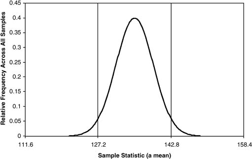
Figure 1 A Sampling Distribution
NOTES: The mean of the sampling distribution (expected value) is 135.0. The two vertical lines represent the mean plus or minus 1.96 standard deviations (the standard deviation is 3.98). Of all the possible estimates that could be obtained, 2.5% of them are less than 127.2, 2.5% are greater than 142.8, and the remaining 95% lie between these values.
Therefore, it is necessary only to estimate the standard deviation of the sampling distribution—more commonly referred to as the standard error of the estimate. However, the normal approximation is not universally good. In particular, certain types of estimates may tend to have a nonsymmetrical sampling distribution. In this situation, other methods must be used to estimate confidence intervals, such as replication methods.
It is important to realize that under a single sample design, different sample statistics will have different sampling distributions. Therefore, even if it is possible to estimate the mean and variance of sampling distributions prior to carrying out a survey, it will rarely be possible to select a design that is optimal for all statistics. Sample designs are typically a compromise, chosen to produce sampling distributions that are likely to be good enough for most of the estimates required.
...
- Analysis of Variance
- Association and Correlation
- Association
- Association Model
- Asymmetric Measures
- Biserial Correlation
- Canonical Correlation Analysis
- Correlation
- Correspondence Analysis
- Intraclass Correlation
- Multiple Correlation
- Part Correlation
- Partial Correlation
- Pearson's Correlation Coefficient
- Semipartial Correlation
- Simple Correlation (Regression)
- Spearman Correlation Coefficient
- Strength of Association
- Symmetric Measures
- Basic Qualitative Research
- Basic Statistics
- F Ratio
- N(n)
- t-Test
- X¯
- Y Variable
- z-Test
- Alternative Hypothesis
- Average
- Bar Graph
- Bell-Shaped Curve
- Bimodal
- Case
- Causal Modeling
- Cell
- Covariance
- Cumulative Frequency Polygon
- Data
- Dependent Variable
- Dispersion
- Exploratory Data Analysis
- Frequency Distribution
- Histogram
- Hypothesis
- Independent Variable
- Measures of Central Tendency
- Median
- Null Hypothesis
- Pie Chart
- Regression
- Standard Deviation
- Statistic
- Causal Modeling
- DISCOURSE/CONVERSATION ANALYSIS
- Econometrics
- Epistemology
- Ethnography
- Evaluation
- Event History Analysis
- Experimental Design
- Factor Analysis and Related Techniques
- Feminist Methodology
- Generalized Linear Models
- HISTORICAL/COMPARATIVE
- Interviewing in Qualitative Research
- Latent Variable Model
- LIFE HISTORY/BIOGRAPHY
- LOG-LINEAR MODELS (CATEGORICAL DEPENDENT VARIABLES)
- Longitudinal Analysis
- Mathematics and Formal Models
- Measurement Level
- Measurement Testing and Classification
- Multilevel Analysis
- Multiple Regression
- Qualitative Data Analysis
- Sampling in Qualitative Research
- Sampling in Surveys
- Scaling
- Significance Testing
- Simple Regression
- Survey Design
- Time Series
- ARIMA
- Box-Jenkins Modeling
- Cointegration
- Detrending
- Durbin-Watson Statistic
- Error Correction Models
- Forecasting
- Granger Causality
- Interrupted Time-Series Design
- Intervention Analysis
- Lag Structure
- Moving Average
- Periodicity
- Serial Correlation
- Spectral Analysis
- Time-Series Cross-Section (TSCS) Models
- Time-Series Data (Analysis/Design)
- Trend Analysis
Get a 30 day FREE TRIAL
-
 Watch videos from a variety of sources bringing classroom topics to life
 -
Read modern, diverse business cases
-
Explore hundreds of books and reference titles

Read next

More like this
Sage Recommends
We found other relevant content for you on other Sage platforms.
Have you created a personal profile? Login or create a profile so that you can save clips, playlists and searches