
Entry
Reader's guide
Entries A-Z
Regression Plane
The regression (hyper) plane represents the projection of the dependent variable into the Euclidean subspace spanned by the independent variables.
MULTIPLE REGRESSION using the LEAST SQUARES criterion involves finding the hyperplane that minimizes the sum of squared differences between the observed values of the dependent variable, and the projection of the dependent variable onto that hyperplane.
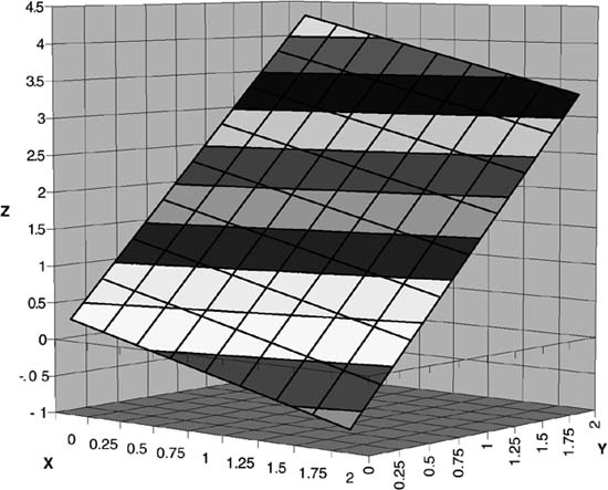
Figure 1 Regression Plane
The hyperplane that minimizes this difference is called the regression hyperplane.
An example clarifies the concept. Suppose that a researcher is interested in the (linear) relationship between the dependent variable Z and the independent variables X and Y. The equation of interest is therefore

Consider the nature of the data being fitted—each observation i defines a point in the three-dimensional space (Xi,Yi,Zi). Intuitively, in the above example, the regression plane is the two-dimensional flat surface that “best fits” the set of three-dimensional data points—where “best fits” means that the regression plane minimizes the sum of squared differences (i.e., residuals) between the surface of the plane (which represents the predicted value of Z given X and Y) and the observed Y. For this example, the regression plane defines the two-dimensional plane that minimizes the sum of squared residuals between the independent variable Z and the plane. More generally, if there are k dependent variables (excluding the constant term), the regression hyperplane is the k-dimensional flat surface representing the best linear projection of Y into the(k +1)-dimensional space spanned by the k independent variables plus the dependent variable. The regression plane is a special case for k = 2.
REGRESSION COEFFICIENTS define the slope of the regression plane in the dimension defined by the respective independent variable. For example, in the three-space defined above, b0 defines the “height” of the regression plane in the third (i.e., Z) dimension when X = Y = 0,b1 defines the slope of the regression plane in the first dimension (i.e., the angle at which the plane intersects the Z-X plane), and b2 defines the slope of the regression plane in the second dimension (i.e., the angle at which the plane intersects the Z-Y plane). The equation for the regression plane is b0 + b1X + b2Y. In other words, just as simple regression involves finding the best fitting line, the generalization to multiple regression involves finding the best fitting plane.
An illustration clarifies. The plane depicted in Figure 1 is characterized by the regression equation Z =0.3 − 0.5X + 2Y. Because the regression plane describes the mapping of Z onto X and Y, it is possible to generate a predicted value of Z for any (X, Y) pair. The regression plane depicts these predictions. The geometric interpretation of the slope coefficients is also evident from the figure. The regression coefficient for X of −0.5 implies that the plane in the figure “tilts” to the left; higher values of X lead to lower predicted values of Z. In contrast, the plane “rises” in the back because the slope coefficient for Y is positive. The intercept (in this case, 0.3) is given by the “height” of the plane when X = Y = 0.
...
- Analysis of Variance
- Association and Correlation
- Association
- Association Model
- Asymmetric Measures
- Biserial Correlation
- Canonical Correlation Analysis
- Correlation
- Correspondence Analysis
- Intraclass Correlation
- Multiple Correlation
- Part Correlation
- Partial Correlation
- Pearson's Correlation Coefficient
- Semipartial Correlation
- Simple Correlation (Regression)
- Spearman Correlation Coefficient
- Strength of Association
- Symmetric Measures
- Basic Qualitative Research
- Basic Statistics
- F Ratio
- N(n)
- t-Test
- X¯
- Y Variable
- z-Test
- Alternative Hypothesis
- Average
- Bar Graph
- Bell-Shaped Curve
- Bimodal
- Case
- Causal Modeling
- Cell
- Covariance
- Cumulative Frequency Polygon
- Data
- Dependent Variable
- Dispersion
- Exploratory Data Analysis
- Frequency Distribution
- Histogram
- Hypothesis
- Independent Variable
- Measures of Central Tendency
- Median
- Null Hypothesis
- Pie Chart
- Regression
- Standard Deviation
- Statistic
- Causal Modeling
- DISCOURSE/CONVERSATION ANALYSIS
- Econometrics
- Epistemology
- Ethnography
- Evaluation
- Event History Analysis
- Experimental Design
- Factor Analysis and Related Techniques
- Feminist Methodology
- Generalized Linear Models
- HISTORICAL/COMPARATIVE
- Interviewing in Qualitative Research
- Latent Variable Model
- LIFE HISTORY/BIOGRAPHY
- LOG-LINEAR MODELS (CATEGORICAL DEPENDENT VARIABLES)
- Longitudinal Analysis
- Mathematics and Formal Models
- Measurement Level
- Measurement Testing and Classification
- Multilevel Analysis
- Multiple Regression
- Qualitative Data Analysis
- Sampling in Qualitative Research
- Sampling in Surveys
- Scaling
- Significance Testing
- Simple Regression
- Survey Design
- Time Series
- ARIMA
- Box-Jenkins Modeling
- Cointegration
- Detrending
- Durbin-Watson Statistic
- Error Correction Models
- Forecasting
- Granger Causality
- Interrupted Time-Series Design
- Intervention Analysis
- Lag Structure
- Moving Average
- Periodicity
- Serial Correlation
- Spectral Analysis
- Time-Series Cross-Section (TSCS) Models
- Time-Series Data (Analysis/Design)
- Trend Analysis
Get a 30 day FREE TRIAL
-
 Watch videos from a variety of sources bringing classroom topics to life
 -
Read modern, diverse business cases
-
Explore hundreds of books and reference titles

Read next

More like this
Sage Recommends
We found other relevant content for you on other Sage platforms.
Have you created a personal profile? Login or create a profile so that you can save clips, playlists and searches