Regression Diagnostics

Common violations of the assumptions of least squares regression are nonlinearity, HETEROSKEDASTICITY, and non-normally distributed error terms. Unusual observations can also have undue influence on the regression equation, and MULTICOLLINEARITY can cause unstable estimates. It is important to perform diagnostics of the model because if these problems are not rectified, OLS estimates are no longer the BEST LINEAR UNBIASED ESTIMATORS.

Nonlinearity in simple regression is easily assessed by examining a SCATTERPLOT of the dependent variable Y against the independent variable X. In multiple regression, however, simple scatterplots no longer suffice because they show only the marginal relationships between Y and each of the individual Xs, when the model gives partial regression coefficients. Partial residual plots (also called component-plus residual plots) are thus used to assess linearity in the [Page 940]multivariate case. The partial residual E(j), for the jth independent variable, is simply the linear component of the partial regression of Y on Xj added to the least squares residuals. The E(j) are plotted versus Xj, and linearity is assessed in the same manner as the scatterplot for simple regression.

Nonlinear relationships can be handled by transforming Y and/or X (when the nonlinearity is simple and monotone), POLYNOMIAL EQUATIONS (when the relationship is nonmonotone but has relatively few changes in direction), or LOCAL REGRESSION (when the nonlinear relationship is very complex).

Unusual observations that are OUTLIERS (i.e., have an unusual Y value given their X value) and have high leverage (characterized by an unusual X value) unduly influence the coefficients of a regression model.

Statistical tests for outliers are usually based on the studentized residuals (sometimes called standardized residuals). The “mean shift” regression model—which simply includes a DUMMY VARIABLE coded 1 for the unusual observation and 0 for all other cases—is a commonly used method for finding the studentized residual for an outlier. If the coefficient for the dummy variable is statistically significant, the observation significantly deviates from the pattern of the rest of the data. Nevertheless, because we select the furthest outlier, rather than observations at random, a simple t-test is inappropriate. A Bonferroni adjustment to the p value remedies this problem. The Bonferroni p value for the largest outlier is p = 2np', where p' is the unadjusted p value from a t-test with n−k −2 degrees of freedom.

Leverage is measured by the hat value hi, which captures how much the observed Yi affects the predicted value ^Y. In simple regression, hat values are determined by hi = Σj=1 (Xj − X¯)2 and are bounded between 1/n and 1, with an average of (k + 1)/n. Hat values that are approximately twice the average are usually considered noteworthy.

The most commonly used diagnostic for INFLUENTIAL CASES is Cook’s Distance (or, more simply, Cook’s D) which measures the impact of an unusual observation on the slope coefficient. Cook’s Dissimply calculated:

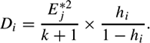
There is no universally accepted cutoff for Cook’s D, but a loose rule of thumb is that values greater than 4/(n − k − 1) should be looked at closely.

...