Probit Analysis

Probit analysis originated as a method of analyzing quantal (dichotomous) responses. Quantal responses involve situations in which there is only one possible response to a stimulus, sometimes referred to as “all-or-nothing.” Early applications of probit analysis involved biological assays. A classic example involves the determination of death when an insect is exposed to an insecticide. Although theoretically the health of the insect deteriorates as exposure to the insecticide is increased, measurement limitations or focus on a specific result necessitate the use of a dichotomous variable to represent the quantal response. Current applications in the social sciences often involve individual-level behavior such as whether a member of Congress votes for or against a bill or when a judge affirms or reverses a lower court decision.

Analytical work in the social sciences often uses a form of linear regression analysis (e.g., ordinary least squares [OLS]). A fundamental assumption of regression analysis is that the dependent variable is continuous, which allows for a linear model. Many research questions, however, involve situations with a dichotomous dependent variable (such as the decision making of human actors, with a prime example being individual voting behavior). Because certain regression assumptions are violated when the dependent variable is dichotomous, which in turn may lead to serious errors of inference, analysis of dichotomous variables generally requires a nonlinear estimation procedure, and probit is a common choice.

The conceptual approach of regression is to estimate the coefficients for a linear model that minimizes the sum of the squared errors between the observed and predicted values of the dependent variable given the values of the independent variables. In contrast, the approach of probit is to estimate the coefficients of a nonlinear model that maximizes the likelihood of observing the value of the dependent variable given the values of the independent variables. As such, probit estimates are obtained by the method known as maximum likelihood estimation.

The probit model makes four basic assumptions. First, the error term is normally distributed. With this assumption, the probit estimates have a set of properties similar to those of OLS estimates (e.g., unbiasedness, normal sampling distributions, minimum variance). Second, the probability that the dependent variable takes on the value 1 (given the choices 0 and 1) is a function of the independent variables. Third, the observations of the dependent variable are statistically independent. This rules out serial correlation. Fourth, there are no perfect linear dependencies among the independent variables. As with OLS, near but not exact linear dependencies may result in multicollinearity.

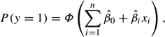
Although probit estimates appear similar to those of OLS regression, their interpretation is less straightforward. Probit estimates are probabilities of observing a 0 or 1 in the dependent variable given the values of the independent variables for a particular observation. The coefficient estimate for each independent variable is the amount the probability of the dependent variable taking on the value 1 increases (or decreases if the estimate is negative), and it is given in standard deviations, a Z-score, based on the cumulative normal probability distribution. Thus, the estimated probability that y = 1 for a given observation is

...