Normalization

In many popular statistical models, we assume that some component of a variable Y has a NORMAL DISTRIBUTION. For example, in the linear regression model Y = α + βX + ε, we typically assume that the error term ε is normal. Although minor departures from normality may be acceptable, distributions with heavier-than-normal tails can compromise statistical estimates. In such cases, it may be preferable to transform Y so that the pertinent component is closer to normality. Transforming a variable in this way is called normalization.

If the pertinent component of Y has one heavy tail (skewed), then we often apply a power transformation. True to their name, power transformations raise Y to some power p (i.e., they transform Y into Yp). Powers greater than 1 reduce negative skew: An example is the quadratic transformation Y 2(p = 2). Powers between 0 and 1 reduce positive skew: An example is the square-root transformation or √Y or √Y + 1/2 (p = 0.5), which is common when Y represents counts or frequencies. For a power of 0, the power transformation is defined to be log(Y), which reduces positive skew in much the same way as a very small power. Negative powers have the same effect as positive powers applied to the reciprocal 1/Y and are used when the reciprocal has a natural interpretation—as when Y is a rate (events per unit time), so that 1 Y is the time between events.

In sum, the family of power transformations can be written as follows:

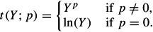
Power transformations assume that Y is positive; if Y can be zero or negative, we commonly make Y positive by adding a constant. There are formal procedures for estimating the best constant to add, as well as the power p that yields the best approximation to normality (Box & Cox, 1964). However, the optimal power and additive constant are usually treated only as rough guidelines.

If the pertinent component of Y has two heavy tails (excess KURTOSIS), we may use a modulus transformation (John & Draper, 1980),

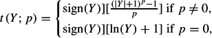
which is a modified power transformation applied to each tail separately. Non-negative powers p less than 1 reduce kurtosis, while powers greater than 1 increase kurtosis. Again, there are formal procedures for estimating the optimal power p (John & Draper, 1980). If Y is symmetric around 0, then the modulus transformation will change the kurtosis without introducing skew. If Y is not centered at 0, it may be advisable to add a constant before applying the modulus transformation.

Other normalizations are typically used if Y represents proportions between 0 and 1: the arcsine or angular transformation sin−1(√Y), the logit or logistic transformation , and the probit transformation Φ−1 (Y) where Φ−1 is the inverse of the cumulative standard normal density. The logit and probit are better normalizations than the arcsine, which is gradually disappearing from practice.

Even the best transformation may not provide an adequate approximation to normality. Moreover, a transformed variable may be hard to interpret, and conclusions drawn from it may not apply to the original, untransformed variable (Levin, Liukkonen, & Levine, 1996). Fortunately, modern researchers often have good alternatives to normalization. When working with non-normal data, we can use a GENERALIZED LINEAR MODEL that assumes a different type of distribution. Or we can make weaker assumptions by using statistics that are “distribution-free” or nonparametric.

...