
Entry
Reader's guide
Entries A-Z
Normal Distribution
The normal distribution (sometimes referred to as the Gaussian distribution) has been applied to problems in the social sciences many times. Many continuous random variables can be modeled as a normal PROBABILITY distribution whose density function produces a symmetric, bell-shaped curve. The normal density function for a continuous random variable Y is

where −∞ <y< ∞, −∞ <µ< ∞, and σ> 0, and µ and σ are the POPULATION mean and STANDARD DEVIATION, respectively, such that E(Y) = µ, and V(Y) = σ2. Notice that these are the only two PARAMETERS that define the density of the normal distribution.
The normal distribution has a special property that holds across parameter values: 68% of the distribution lies within 1 standard deviation above and below the mean, 95% of the distribution lies within 2 standard deviations above and below the mean, and 99.7% of the distribution lies within 3 standard deviations of the mean. However, because the distribution lies between −∞ and ∞, a normally distributed random variable has events with nonzero probability occurring anywhere on the real-number line. In addition, because the distribution is symmetric and has a unique maximum, its MEAN, MEDIAN, and MODE are the same. Furthermore, the two inflection points are located 1 standard deviation away from the mean. Figures 1 and 2 demonstrate these points. Note that the two distributions are both centered around 3, but the spread of the first is greater than that of the second. However, a very high or very low number is a possible event (even with very low probability) in both distributions.

Figure 1Yi ∼ Normal, µ = 3, σ = 2
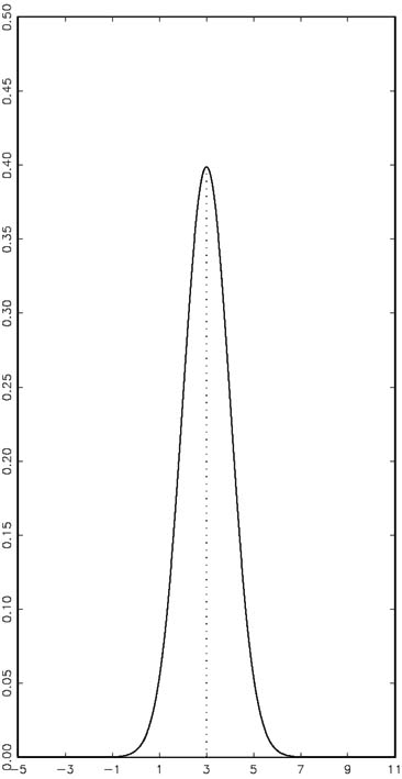
Figure 2Yi ∼ Normal, µ = 3, σ = 1
A major reason for the centrality of the normal distribution in the social sciences is the CENTRAL LIMIT THEOREM. The theorem links any probability function (as long as its µ and σ are finite) to the normal distribution by proving that regardless of the distribution of the original variable, the mean and the sum of the variable are normally distributed for large enough SAMPLES (or, more strictly, as n approaches infinity). A particular application of the theorem is the normal approximation to the BINOMIAL distribution. The application establishes that a fraction of successes in a series of nBERNOULLI trials with a probability of success in each one, p, is approximately normally distributed with a mean p and variance p(1−p)/n .
In addition, following the ASSUMPTION that the ERROR terms in the frequently used LEAST SQUARES REGRESSION are distributed normally, the least squares estimators are distributed normally, a property that helps with many questions of STATISTICAL INFERENCE.
The Standard Normal Distribution
To compare values of two normally distributed variables, each drawn from a different normal distribution, a standardization is required. The standardization shifts the means of the distributions and adjusts their variances to comparable grounds, such that a comparison of, say, a grade in Advanced Akkadian and a grade in Introduction to Astrophysics is made possible.
The standardization procedure is Zi =Yi−µ/σ, such that each value Zi represents the difference from Yi to its mean in units of its standard deviation (σ) of the original variable Yi. Therefore, the mean value of Zi must be zero, and the standard deviation is equal to 1.
...
- Analysis of Variance
- Association and Correlation
- Association
- Association Model
- Asymmetric Measures
- Biserial Correlation
- Canonical Correlation Analysis
- Correlation
- Correspondence Analysis
- Intraclass Correlation
- Multiple Correlation
- Part Correlation
- Partial Correlation
- Pearson's Correlation Coefficient
- Semipartial Correlation
- Simple Correlation (Regression)
- Spearman Correlation Coefficient
- Strength of Association
- Symmetric Measures
- Basic Qualitative Research
- Basic Statistics
- F Ratio
- N(n)
- t-Test
- X¯
- Y Variable
- z-Test
- Alternative Hypothesis
- Average
- Bar Graph
- Bell-Shaped Curve
- Bimodal
- Case
- Causal Modeling
- Cell
- Covariance
- Cumulative Frequency Polygon
- Data
- Dependent Variable
- Dispersion
- Exploratory Data Analysis
- Frequency Distribution
- Histogram
- Hypothesis
- Independent Variable
- Measures of Central Tendency
- Median
- Null Hypothesis
- Pie Chart
- Regression
- Standard Deviation
- Statistic
- Causal Modeling
- DISCOURSE/CONVERSATION ANALYSIS
- Econometrics
- Epistemology
- Ethnography
- Evaluation
- Event History Analysis
- Experimental Design
- Factor Analysis and Related Techniques
- Feminist Methodology
- Generalized Linear Models
- HISTORICAL/COMPARATIVE
- Interviewing in Qualitative Research
- Latent Variable Model
- LIFE HISTORY/BIOGRAPHY
- LOG-LINEAR MODELS (CATEGORICAL DEPENDENT VARIABLES)
- Longitudinal Analysis
- Mathematics and Formal Models
- Measurement Level
- Measurement Testing and Classification
- Multilevel Analysis
- Multiple Regression
- Qualitative Data Analysis
- Sampling in Qualitative Research
- Sampling in Surveys
- Scaling
- Significance Testing
- Simple Regression
- Survey Design
- Time Series
- ARIMA
- Box-Jenkins Modeling
- Cointegration
- Detrending
- Durbin-Watson Statistic
- Error Correction Models
- Forecasting
- Granger Causality
- Interrupted Time-Series Design
- Intervention Analysis
- Lag Structure
- Moving Average
- Periodicity
- Serial Correlation
- Spectral Analysis
- Time-Series Cross-Section (TSCS) Models
- Time-Series Data (Analysis/Design)
- Trend Analysis
Get a 30 day FREE TRIAL
-
 Watch videos from a variety of sources bringing classroom topics to life
 -
Read modern, diverse business cases
-
Explore hundreds of books and reference titles

Read next

More like this
Sage Recommends
We found other relevant content for you on other Sage platforms.
Have you created a personal profile? Login or create a profile so that you can save clips, playlists and searches