
Entry
Reader's guide
Entries A-Z
Logistic Regression
The situation in which the outcome variable (Y) is limited to two discrete values—an event occurring or not occurring, with a “yes” or “no” response to an attitude question, or a characteristic being present or absent, usually coded as 1 or 0 (or 1 or 2), respectively—is quite typical in many areas of social science research, as in dropping out of high school, getting a job, joining a union, giving birth to a child, voting for a certain candidate, or favoring the death penalty. Logistic regression is a common tool for statistically modeling these types of discrete outcomes.
The overall framing and many of the features of the technique are largely analogous to ordinary least squares (OLS) REGRESSION, especially the linear probability model. Many of the warnings and recommendations, including the diagnostics, made for OLS regression apply as well. It is, however, based on a different, less stringent, set of statistical assumptions to explicitly take into account the limited nature of the outcome variable and the problems resulting from it—because the outcome variable as a function of independent variables can take only two values; the error terms are not continuous, homoskedastic, or normally distributed; and the predicted probabilities are not constrained to behave linearly and not to be greater than 1 and less than 0.
Logistic regression fits a special s-shaped curve by taking a linear combination of the explanatory variables and transforming it by a logistic function (cf. probit analysis) as follows:

where p is the probability that the value of the outcome variable is 1, and BX stands for b1x1 + b2x2 +···+ bnxn. The model hence estimates the logit, which is the natural log of the odds of the outcome variable being equal to 1 (i.e., the event occurring, the response being affirmative, or the characteristic being present) or 0 (i.e., the event not occurring, the response being negative, or the characteristic being absent). The probability that the outcome variable is equal to 1 is then the following:

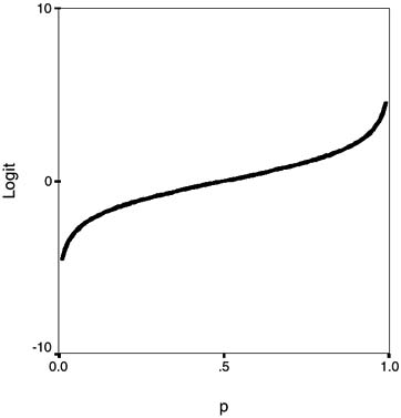
Figure 1 The Relationship Between p and Its Logit
Note that there is a nonlinear relationship between p and its logit, which is illustrated in Figure 1: In the mid-range of p there is a (near) linear relationship, but as p approaches the extremes—0 or 1—the relationship becomes nonlinear with increasingly larger changes in logit for the same change in p.
For large samples, the parameters estimated by MAXIMUM LIKELIHOOD ESTIMATION (MLE) are unbiased, efficient, and normally distributed, thus allowing statistical tests of significance. The technique can be extended to situations involving outcome variables with three or more categories (polytomous, or multinomial dependent variables).
Example
To illustrate its application and the interpretation of the results, we use the data on the attitude toward capital punishment—“Do you favor or oppose the death penalty for persons convicted of murder?”—from the General Social Survey. Out of 2,599 valid responses in 1998, 1,906 favored (73.3%) and 693 opposed (26.7%) it. The analysis below examines the effects of race (White = 1 and non-White = 0) and education on the dependent variable, which is coded as 1 for those who favor it and 0 for those who oppose it, controlling for sex (male = 1 and female = 0) and age.
...
- Analysis of Variance
- Association and Correlation
- Association
- Association Model
- Asymmetric Measures
- Biserial Correlation
- Canonical Correlation Analysis
- Correlation
- Correspondence Analysis
- Intraclass Correlation
- Multiple Correlation
- Part Correlation
- Partial Correlation
- Pearson's Correlation Coefficient
- Semipartial Correlation
- Simple Correlation (Regression)
- Spearman Correlation Coefficient
- Strength of Association
- Symmetric Measures
- Basic Qualitative Research
- Basic Statistics
- F Ratio
- N(n)
- t-Test
- X¯
- Y Variable
- z-Test
- Alternative Hypothesis
- Average
- Bar Graph
- Bell-Shaped Curve
- Bimodal
- Case
- Causal Modeling
- Cell
- Covariance
- Cumulative Frequency Polygon
- Data
- Dependent Variable
- Dispersion
- Exploratory Data Analysis
- Frequency Distribution
- Histogram
- Hypothesis
- Independent Variable
- Measures of Central Tendency
- Median
- Null Hypothesis
- Pie Chart
- Regression
- Standard Deviation
- Statistic
- Causal Modeling
- DISCOURSE/CONVERSATION ANALYSIS
- Econometrics
- Epistemology
- Ethnography
- Evaluation
- Event History Analysis
- Experimental Design
- Factor Analysis and Related Techniques
- Feminist Methodology
- Generalized Linear Models
- HISTORICAL/COMPARATIVE
- Interviewing in Qualitative Research
- Latent Variable Model
- LIFE HISTORY/BIOGRAPHY
- LOG-LINEAR MODELS (CATEGORICAL DEPENDENT VARIABLES)
- Longitudinal Analysis
- Mathematics and Formal Models
- Measurement Level
- Measurement Testing and Classification
- Multilevel Analysis
- Multiple Regression
- Qualitative Data Analysis
- Sampling in Qualitative Research
- Sampling in Surveys
- Scaling
- Significance Testing
- Simple Regression
- Survey Design
- Time Series
- ARIMA
- Box-Jenkins Modeling
- Cointegration
- Detrending
- Durbin-Watson Statistic
- Error Correction Models
- Forecasting
- Granger Causality
- Interrupted Time-Series Design
- Intervention Analysis
- Lag Structure
- Moving Average
- Periodicity
- Serial Correlation
- Spectral Analysis
- Time-Series Cross-Section (TSCS) Models
- Time-Series Data (Analysis/Design)
- Trend Analysis
Get a 30 day FREE TRIAL
-
 Watch videos from a variety of sources bringing classroom topics to life
 -
Read modern, diverse business cases
-
Explore hundreds of books and reference titles

Read next

More like this
Sage Recommends
We found other relevant content for you on other Sage platforms.
Have you created a personal profile? Login or create a profile so that you can save clips, playlists and searches