
Entry
Reader's guide
Entries A-Z
Forecasting
It is far better to foresee even without certainty than not to foresee at all.
Exponential Smoothing Procedures
One can distinguish three basic procedures: simple exponential smoothing for series without trend, Holt’s exponential smoothing for data exhibiting trend, and Winters exponential smoothing for data that include trend and seasonal components.
Simple Exponential Smoothing
An intuitive approach to the prediction of a series without trend is to use the historic average as prediction for all future periods. That is,

Equal weighting of the observations, irrespective of their age, requires stability of the series over time. Because most data series lack this stability, it is better to either average observations over a short, recent time window, or consider a weighted average that discounts observations according to their age. Simple exponential smoothing uses an exponential (geometric) weighted average:

Ln is the estimate of the level at time n. It becomes the forecast of all future observations. The smoothing constant α(0 ≤α≤ 1) gives more weight to recent observations and less weight to observations in the past. When α = 1, the forecast ^yn(r) = Ln = yn makes use of the last observation only. It is called the “naïve” or “random walk” forecast. When α approaches 0, the resulting forecast ^yn(r) = Ln = (yn + yn−1 puts equal weight on all observations.
The level is updated according to Ln = αyn + (1 − α)Ln−1; only the last observation and the previous level estimate need to be stored. This is important if many series must be predicted. It is common to start the recursion at the beginning of the series, with a certain starting value for the level at Time 1. Typically, one uses the first observation (L1 = y1), or an average of the first few observations. From this starting value, one calculates L2 = αy2 + (1 − α)L1, L3 = αy3 + (1 − α)L2, …, until one reaches Ln = αyn + (1 − α)Ln−1. The last level estimate becomes the forecast of all future observations: ^yn(r) = Ln.
The calculations require a value for the smoothing constant. The smoothing constant is estimated by minimizing the sum of the squared one-step-ahead forecast errors,

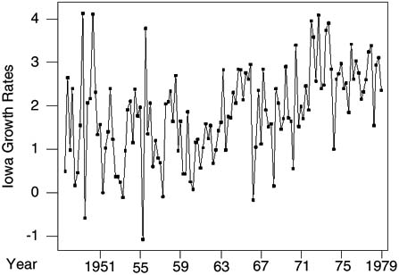
Figure 1 Quarterly Iowa Growth Rates (1948 through 1979)
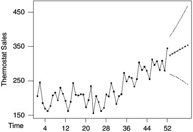
Figure 2 Observations, Forecasts, and 95% Forecast
We illustrate simple exponential smoothing with the quarterly Iowa nonfarm growth rates in Figure 1. The data (n = 127; from 1948/2 through 1979/4) were first analyzed in Abraham and Ledolter (1983). The time series graph shows no obvious trends, but indicates that the level of the series shifts with time. Table 1 illustrates the calculations with smoothing constant α = 0.1. The iterations start with L1 = y1 =0.50. Repeated use of the updating equation gives L2 = (0.1)(2.65) + (0.9)(0.5) = 0.715, L3 = (0.1)(0.97) + (0.9)(0.715) = 0.741, until L127 = (0.1)(2.35) + (0.9)(2.681) = 2.648. Forecasts of all future observations are given by ^y127(r) = 2.648. The one-step-ahead forecast errors are given in the fifth column: y2 − ^y1(1) = 2.65 − 0.50 = 2.15, y3 − ^y2(1) = 0.97 − 0.715 = 0.255, …, y127 − ^y126 (1) = 2.35 − 2.681 =−0.331; the sum of their squares is SSE = 122.61. The sum of squares depends on the smoothing constant, because a different α implies different forecasts. In this example, any smoothing constant different from 0.1 increases the sum of the squared one-step-ahead forecast errors.
...
- Analysis of Variance
- Association and Correlation
- Association
- Association Model
- Asymmetric Measures
- Biserial Correlation
- Canonical Correlation Analysis
- Correlation
- Correspondence Analysis
- Intraclass Correlation
- Multiple Correlation
- Part Correlation
- Partial Correlation
- Pearson's Correlation Coefficient
- Semipartial Correlation
- Simple Correlation (Regression)
- Spearman Correlation Coefficient
- Strength of Association
- Symmetric Measures
- Basic Qualitative Research
- Basic Statistics
- F Ratio
- N(n)
- t-Test
- X¯
- Y Variable
- z-Test
- Alternative Hypothesis
- Average
- Bar Graph
- Bell-Shaped Curve
- Bimodal
- Case
- Causal Modeling
- Cell
- Covariance
- Cumulative Frequency Polygon
- Data
- Dependent Variable
- Dispersion
- Exploratory Data Analysis
- Frequency Distribution
- Histogram
- Hypothesis
- Independent Variable
- Measures of Central Tendency
- Median
- Null Hypothesis
- Pie Chart
- Regression
- Standard Deviation
- Statistic
- Causal Modeling
- DISCOURSE/CONVERSATION ANALYSIS
- Econometrics
- Epistemology
- Ethnography
- Evaluation
- Event History Analysis
- Experimental Design
- Factor Analysis and Related Techniques
- Feminist Methodology
- Generalized Linear Models
- HISTORICAL/COMPARATIVE
- Interviewing in Qualitative Research
- Latent Variable Model
- LIFE HISTORY/BIOGRAPHY
- LOG-LINEAR MODELS (CATEGORICAL DEPENDENT VARIABLES)
- Longitudinal Analysis
- Mathematics and Formal Models
- Measurement Level
- Measurement Testing and Classification
- Multilevel Analysis
- Multiple Regression
- Qualitative Data Analysis
- Sampling in Qualitative Research
- Sampling in Surveys
- Scaling
- Significance Testing
- Simple Regression
- Survey Design
- Time Series
- ARIMA
- Box-Jenkins Modeling
- Cointegration
- Detrending
- Durbin-Watson Statistic
- Error Correction Models
- Forecasting
- Granger Causality
- Interrupted Time-Series Design
- Intervention Analysis
- Lag Structure
- Moving Average
- Periodicity
- Serial Correlation
- Spectral Analysis
- Time-Series Cross-Section (TSCS) Models
- Time-Series Data (Analysis/Design)
- Trend Analysis
Get a 30 day FREE TRIAL
-
 Watch videos from a variety of sources bringing classroom topics to life
 -
Read modern, diverse business cases
-
Explore hundreds of books and reference titles

Read next

More like this
Sage Recommends
We found other relevant content for you on other Sage platforms.
Have you created a personal profile? Login or create a profile so that you can save clips, playlists and searches