Dispersion

Dispersion roughly refers to the degree of scatter or variability in a collection of observations. For example, individuals might differ about whether a political leader is doing a good job; children might respond differently to a method aimed at enhancing reading; and even in the physical sciences, measurements might differ from one occasion to the next because of the imprecision of the instruments used. In a very real sense, it is dispersion that motivates interest in statistical techniques.

A basic issue is deciding how dispersion should be measured when trying to characterize a population of individuals or things. That is, if all individuals of interest could be measured, how should the variation among these individuals be characterized? Such measures are population measures of dispersion. A related issue is deciding how to estimate a population measure of dispersion based on a sample of individuals.

Choosing a measure of dispersion is a complex issue that has seen many advances during the past 30 years. The choice depends in part on the goal of the investigator, with the optimal choice often changing drastically depending on what an investigator wants to know or do. More than 150 measures of dispersion have been proposed, comparisons of which were made by Lax (1985) based on some fundamental criteria that are relevant to a range of practical problems. Although most of these measures seem to have little practical value, at least five or six play an important and useful role.

Certainly the best known measure of dispersion is the population variance, which is typically written as σ2. It is the average (or expected) value of the squared difference between an observation and the population mean, μ. That is, if all individuals could be measured, the average of their responses is called the population mean, μ, and if, for every observation, the squared difference between it and μ were computed, the average of these squared values is σ2. In more formal terms, σ2 = E(X − μ)2, where X is any observation we might make and E stands for expected value. The (positive) square root of σ2, σ is called the (population) standard deviation. Based on a sample of n individuals, if we observe the values X1,…, Xn, the usual estimate of σ2 is the sample variance:

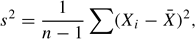
where X¯ = ∑Xi/n is the sample mean.

For some purposes, the use of the standard deviation, σ, stems from the fundamental result that the probability of an observation being within some specified distance from the mean, as measured by σ, is completely determined under normality. For example, the probability that an observation is within 1 standard deviation of the mean is 0.68, and the probability of being within 2 standard deviations is 0.954. These properties have led to a commonly used measure of effect size (a measure intended to characterize the extent to which two groups differ) as well as a frequently employed rule for detecting outliers (unusually large or small values). Shortly after a seminal paper by Tukey (1960), it was realized that even very small departures from normality can alter these properties substantially, resulting in practical problems that commonly occur.

...