
Entry
Reader's guide
Entries A-Z
Commonality Analysis
Commonality analysis is a method used to partition the explained/predicted variance in either a measured or a latent variable into subcomponents explained (a) uniquely by each measured predictor variable and (b) in common by every possible combination of the PREDICTOR VARIABLES. The explained variance and all the subcomponents of the explained variance are each in a squared, variance-accounted-for metric. Commonality analysis was originally developed for use in REGRESSION but also can be applied in other MULTIVARIATE ANALYSES (cf. Frederick, 1999).
Heuristic Example
To make the discussion concrete, presume a regression problem involving a single measured outcome variable (Y) and two predictor variables (X1 and X2). The results associated with the example are presented graphically in the Venn diagram in Figure 1.
In this example, each of the three measured variables has a sum of squares (SOS) of 400, corresponding to the box for each measured variable being drawn as encompassing 20 × 20 units of area. As regards the overlap of X1 and Y, because 100 units of the SOSY = 400 are predicted by X1, the r2YX1 = 100/400 = .2500 = 25.00%. X2 explains 225 of the 400 units of Y, and so the r2YX2 = 225/400 = .5625 = 56.25%.
However, the multiple CORRELATION SQUARED (R2[YX1X2]) does not equal 25.00% plus 56.25%, or 81.25%, because the predictors are correlated (r2X1X2 = 18.75%). Therefore, some of the explanatory power of X1 and X2 is common to both and should not be “double counted” in computing R2[YX1X2]. For this example, X1 and X2 together explain R2[YX1X2] = 68.75% of the variability in the Y scores (and not 81.25%).
But where does this 68.75% effect size originate? The following questions must be addressed:
- How much of the observed effect size is due to the unique explanatory power of X1?
- How much of the observed effect size is due to the unique explanatory power of X2?
- How much of the observed effect size is due to the common explanatory power of X1 and X2?
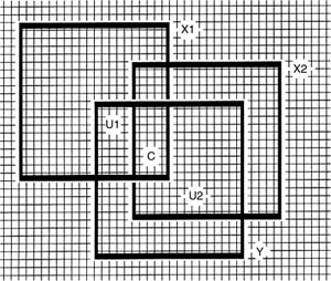
Figure 1 Venn Diagram for a Two-Predictor Regression Commonality Analysis
These are the questions addressed in a commonality analysis.
The analysis is conducted in a series of four steps. First, the R2 is computed using all possible combinations of the predictor variables. For this simple example, there are only three possible combinations, and R2[YX1X2] = 68.75%, R2[YX1] = 25.00%, and R2[YX2] = 56.25%.
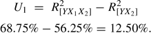
Second, values obtained in Step 1 are inserted into commonality analysis formulas provided in various publications (cf. Rowell, 1996). For this example, the unique predictive contribution (U1)of X1 is computed as
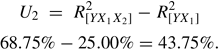
The unique contribution (U2)of X2 is computed as
The common contribution (C12)of X1 and X2 is computed as

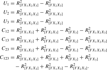
The commonality analysis computational formulas become exponentially more complicated as there are more predictor variables (Rowell, 1996). For example, when there are three predictor variables, the formulas are as follows:
Third, as a check on the computations, the R2[YX1X2] is recomputed as

...
- Analysis of Variance
- Association and Correlation
- Association
- Association Model
- Asymmetric Measures
- Biserial Correlation
- Canonical Correlation Analysis
- Correlation
- Correspondence Analysis
- Intraclass Correlation
- Multiple Correlation
- Part Correlation
- Partial Correlation
- Pearson's Correlation Coefficient
- Semipartial Correlation
- Simple Correlation (Regression)
- Spearman Correlation Coefficient
- Strength of Association
- Symmetric Measures
- Basic Qualitative Research
- Basic Statistics
- F Ratio
- N(n)
- t-Test
- X¯
- Y Variable
- z-Test
- Alternative Hypothesis
- Average
- Bar Graph
- Bell-Shaped Curve
- Bimodal
- Case
- Causal Modeling
- Cell
- Covariance
- Cumulative Frequency Polygon
- Data
- Dependent Variable
- Dispersion
- Exploratory Data Analysis
- Frequency Distribution
- Histogram
- Hypothesis
- Independent Variable
- Measures of Central Tendency
- Median
- Null Hypothesis
- Pie Chart
- Regression
- Standard Deviation
- Statistic
- Causal Modeling
- DISCOURSE/CONVERSATION ANALYSIS
- Econometrics
- Epistemology
- Ethnography
- Evaluation
- Event History Analysis
- Experimental Design
- Factor Analysis and Related Techniques
- Feminist Methodology
- Generalized Linear Models
- HISTORICAL/COMPARATIVE
- Interviewing in Qualitative Research
- Latent Variable Model
- LIFE HISTORY/BIOGRAPHY
- LOG-LINEAR MODELS (CATEGORICAL DEPENDENT VARIABLES)
- Longitudinal Analysis
- Mathematics and Formal Models
- Measurement Level
- Measurement Testing and Classification
- Multilevel Analysis
- Multiple Regression
- Qualitative Data Analysis
- Sampling in Qualitative Research
- Sampling in Surveys
- Scaling
- Significance Testing
- Simple Regression
- Survey Design
- Time Series
- ARIMA
- Box-Jenkins Modeling
- Cointegration
- Detrending
- Durbin-Watson Statistic
- Error Correction Models
- Forecasting
- Granger Causality
- Interrupted Time-Series Design
- Intervention Analysis
- Lag Structure
- Moving Average
- Periodicity
- Serial Correlation
- Spectral Analysis
- Time-Series Cross-Section (TSCS) Models
- Time-Series Data (Analysis/Design)
- Trend Analysis
Get a 30 day FREE TRIAL
-
 Watch videos from a variety of sources bringing classroom topics to life
 -
Read modern, diverse business cases
-
Explore hundreds of books and reference titles

Read next

More like this
Sage Recommends
We found other relevant content for you on other Sage platforms.
Have you created a personal profile? Login or create a profile so that you can save clips, playlists and searches