Cointegration

When a linear combination of nonstationary variables is stationary, the variables are said to be cointegrated, and the vector that defines the stationary linear combination is called a cointegration vector. A [Page 142]time series is stationary if its distribution does not vary over time. The simplest example of a stationary process is {εt} = …,ε-1, ε0, ε1,…., which represents a sequence of independent and identically distributed random variables. The subscript t refers to time. If the distribution of a variable depends on t, it is nonstationary. In cointegration analysis, the most common form of nonstationarity is that of the integrated variables. The random walk, Xt = Xt-1 + εt = X0 + Σti = 1 εi, is an example of a nonstationary variable that is integrated of order one. The word integration refers to the cumulation of epsilons.

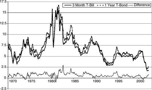
Figure 1 The Interest Rates on a 3-Month Treasury Bill and a 1-Year Treasury Bond for the Period From January 1970 to April 2002

NOTE: The two interest rates appear to be nonstationary, whereas the difference between them seems to be stationary, so the two interest rates are cointegrated.

Federal Reserve Bank of St. Louis.

The concept of cointegration is interesting because it can be applied to uncover relationships that may have theoretical interpretations. For example, the cointegration relations may be defined by the first-order conditions of an economic model, and cointegration analysis can be used to estimate economic models and test certain theoretical hypotheses.

The classical example on cointegration is about a dog that follows its drunk owner. In this example, the positions of the dog and its owner, as a function of time, are two nonstationary processes because the drunk owner is walking around, taking steps in random directions. However, the two processes are cointegrated because the distance between dog and owner is stationary.

Another example is a property of interest rates on bonds with different maturities. Individually, they may have large fluctuations, but the difference between them appears to be stationary. This is illustrated in Figure 1, which contains the interest rates on a 3-month Treasury bill and a 1-year Treasury bond for the period from January 1970 to April 2002. The thin solid line is the difference between the two interest rates.