
Entry
Reader's guide
Entries A-Z
Subject index
Normal Curve Distribution
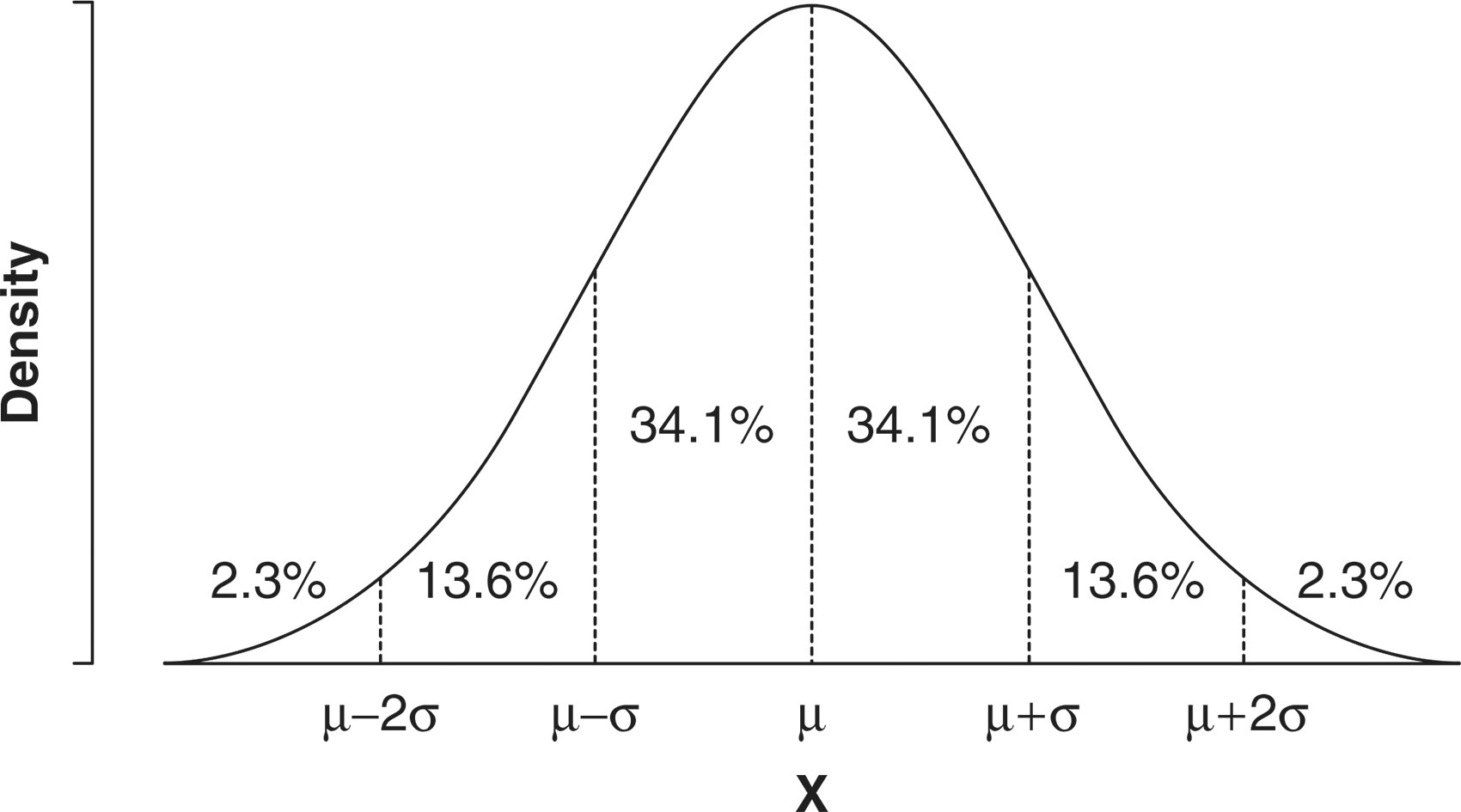
Normal curve distribution is a symmetrical distribution, which has a bell shape and identical scores for the mean (i.e., the average score), median (i.e., the middle score splitting the bottom 50% from the top 50% in the distribution), and mode (i.e., most frequent value). A bell-shaped curve (see an example in Figure 1) characterizing the normal distribution can be represented by the equation below:
where Y = frequency of a given value of X; X = any score in the distribution; µ = mean of the distribution (the mean or the average score is the ratio of the sum of all scores to the number of scores in the distribution); σ = standard deviation of the distribution (standard deviation is one of the variability measures representing the average of the number of scores about the mean); N = the number of data points (or frequency) in the distribution; π = a constant of 3.1416; and e = a constant of 2.7183.
Figure 1 The Normal Curve
For users of statistics who are primarily interested in applying their statistical knowledge in social scientific research to analyze data, Equation 1 is of little practical use. But, it illustrates the notion that the normal curve is a theoretical distribution that can be mathematically represented.
In the curve depicted in Figure 1 each side of the mean has an inflection point, situated where the direction of the curvature changes from curving down to curving up. For any normally distributed bell curve, the inflection points are located 1 standard deviation above and below the mean. At each tail of the distribution, the curve gets close to the x axis, although theoretically, it never touches the horizontal axis. In statistics, such a curve is described as being asymptotic to the horizontal axis.
Relationship Between Mean, Standard Deviation and Area Under the Curve
In any normal distribution, the mean and the standard deviation have a special connection to the area under the curve. In a normally distributed set of scores 34.13% of the area below the curve is located between the mean and 1 standard deviation or µ + 1σ. Furthermore,
- 13.59% of the area is between µ + 1σ and µ + 2σ;
- 2.15% of the area is between µ + 2σ and µ + 3σ; and
- 0.13% of the area can be found above µ + 3σ.
Taken together, these percentages comprise 50% of the area. Because the bell curve is symmetrical, the same relationship between the mean, standard deviation, and the area under the curve applies for scores below the mean.
Let’s consider an example of a population of 10,000 intelligence scores, which is normally distributed with µ = 100 and σ = 16. By applying the aforementioned information about the relationship between the mean, standard deviation, and the area below the curve to this example, one can determine that 34.13% of the scores are located between 100 and 116 ( μ + 1σ = 100 + 16 = 116), 13.59% of the scores are between 116 and 132 (μ + 2σ = 100 + 32 = 132), 2.15% are between 132 and 148, and 0.13% are above 148. Likewise, 34.13% of the scores are located between 84 and 100, 13.59% of scores are between 68 and 84, 2.15% are between 52 and 68, and 0.13% are below 52.
...
- Creating and Conducting Research
- Creation of Research Project
- Authoring: Telling a Research Story
- Body Image and Eating Disorders
- Hypothesis Formulation
- Methodology, Selection of
- Program Assessment
- Research Ideas, Sources of
- Research Project, Planning of
- Research Question Formulation
- Research Topic, Definition of
- Research, Inspiration for
- Social Media: Blogs, Microblogs, and Twitter
- Testability
- Ethics
- Acknowledging the Contribution of Others
- Activism and Social Justice
- Anonymous Source of Data
- Authorship Bias
- Authorship Credit
- Confidentiality and Anonymity of Participants
- Conflict of Interest in Research
- Controversial Experiments
- Copyright Issues in Research
- Cultural Sensitivity in Research
- Data Security
- Debriefing of Participants
- Deception in Research
- Ethical Issues, International Research
- Ethics Codes and Guidelines
- Fraudulent and Misleading Data
- Funding Research
- Health Care Disparities
- Human Subjects, Treatment of
- Informed Consent
- Institutional Review Board
- Organizational Ethics
- Peer Review
- Plagiarism
- Plagiarism, Self-
- Privacy of Information
- Privacy of Participants
- Public Behavior, Recording of
- Reliability, Unitizing
- Research Ethics and Social Values
- Researcher-Participant Relationships
- Social Implications of Research
- Literature Reviews
- Archive Searching for Research
- Bibliographic Research
- Databases, Academic
- Foundation and Government Research Collections
- Library Research
- Literature Review, The
- Literature Reviews, Foundational
- Literature Reviews, Resources for
- Literature Reviews, Strategies for
- Literature Sources, Skeptical and Critical Stance Toward
- Literature, Determining Quality of
- Literature, Determining Relevance of
- Meta-Analysis
- Publications, Scholarly
- Search Engines for Literature Search
- Vote Counting Literature Review Methods
- Writing and Publishing Research
- Abstract or Executive Summary
- Academic Journals
- Alternative Conference Presentation Formats
- American Psychological Association (APA) Style
- Archiving Data
- Blogs and Research
- Chicago Style
- Citations to Research
- Evidence-Based Policy Making
- Invited Publication
- Limitations of Research
- Modern Language Association (MLA) Style
- Narrative Literature Review
- New Media Analysis
- News Media, Writing for
- Panel Presentations and Discussion
- Pay to Review and/or Publish
- Peer Reviewed Publication
- Poster Presentation of Research
- Primary Data Analysis
- Publication Style Guides
- Publication, Politics of
- Publications, Open-Access
- Publishing a Book
- Publishing a Journal Article
- Research Report, Organization of
- Research Reports, Objective
- Research Reports, Subjective
- Scholarship of Teaching and Learning
- Secondary Data
- Submission of Research to a Convention
- Submission of Research to a Journal
- Title of Manuscript, Selection of
- Visual Images as Data Within Qualitative Research
- Writer’s Block
- Writing a Discussion Section
- Writing a Literature Review
- Writing a Methods Section
- Writing a Results Section
- Writing Process, The
- Creation of Research Project
- Designing the Empirical Inquiry
- Content Analysis
- Coding of Data
- Content Analysis, Definition of
- Content Analysis, Process of
- Content Analysis: Advantages and Disadvantages
- Conversation Analysis
- Critical Analysis
- Discourse Analysis
- Interaction Analysis, Quantitative
- Intercoder Reliability
- Intercoder Reliability Coefficients, Comparison of
- Intercoder Reliability Standards: Reproducibility
- Intercoder Reliability Standards: Stability
- Intercoder Reliability Techniques: Cohen’s Kappa
- Intercoder Reliability Techniques: Fleiss System
- Intercoder Reliability Techniques: Holsti Method
- Intercoder Reliability Techniques: Krippendorf Alpha
- Intercoder Reliability Techniques: Percent Agreement
- Intercoder Reliability Techniques: Scott’s Pi
- Metrics for Analysis, Selection of
- Narrative Analysis
- Observational Research Methods
- Observational Research, Advantages and Disadvantages
- Observer Reliability
- Rhetorical and Dramatism Analysis
- Semiotics
- Unobtrusive Analysis
- Internet Inquiry
- Association of Internet Researchers (AoIR)
- Chat Rooms
- Computer-Mediated Communication (CMC)
- Internet as Cultural Context
- Internet Research and Ethical Decision Making
- Internet Research, Privacy of Participants
- Online and Offline Data, Comparison of
- Online Communities
- Online Data, Collection and Interpretation of
- Online Data, Documentation of
- Online Data, Hacking of
- Online Interviews
- Online Social Worlds
- Social Networks, Online
- Spam
- Measurement
- Correspondence Analysis
- Cutoff Scores
- Data Cleaning
- Data Reduction
- Data Trimming
- Facial Affect Coding System
- Factor Analysis
- Factor Analysis-Oblique Rotation
- Factor Analysis: Confirmatory
- Factor Analysis: Evolutionary
- Factor Analysis: Exploratory
- Factor Analysis: Internal Consistency
- Factor Analysis: Parallelism Test
- Factor Analysis: Rotated Matrix
- Factor Analysis: Varimax Rotation
- Implicit Measures
- Measurement Levels
- Measurement Levels, Interval
- Measurement Levels, Nominal/Categorical
- Measurement Levels, Ordinal
- Measurement Levels, Ratio
- Observational Measurement: Face Features
- Observational Measurement: Proxemics and Touch
- Observational Measurement: Vocal Qualities
- Organizational Identification
- Outlier Analysis
- Parsimony
- Physiological Measurement
- Physiological Measurement: Blood Pressure
- Physiological Measurement: Genital Blood Volume
- Physiological Measurement: Heart Rate
- Physiological Measurement: Pupillary Response
- Physiological Measurement: Skin Conductance
- Range
- Raw Score
- Reaction Time
- Reliability of Measurement
- Reliability, Cronbach’s Alpha
- Reliability, Knuder-Richardson
- Reliability, Split-half
- Scales, Forced Choice
- Scales, Likert Statement
- Scales, Open-Ended
- Scales, Rank Order
- Scales, Semantic Differential
- Scales, True/False
- Scaling, Guttman
- Standard Score
- Time Series Notation
- True Score
- Validity, Concurrent
- Validity, Construct
- Validity, Face and Content
- Validity, Halo Effect
- Validity, Measurement of
- Validity, Predictive
- Variables, Conceptualization
- Variables, Operationalization
- Z Transformation
- Research Subjects/Participants
- Sampling
- Survey Research
- Opinion Polling
- Sampling, Random
- Survey Instructions
- Survey Questions, Writing and Phrasing of
- Survey Response Rates
- Survey Wording
- Survey: Contrast Questions
- Survey: Demographic Questions
- Survey: Dichotomous Questions
- Survey: Filter Questions
- Survey: Follow-up Questions
- Survey: Leading Questions
- Survey: Multiple-Choice Questions
- Survey: Negative-Wording Questions
- Survey: Open-Ended Questions
- Survey: Questionnaire
- Survey: Sampling Issues
- Survey: Structural Questions
- Surveys, Advantages and Disadvantages of
- Surveys, Using Others’
- Under-represented Group
- Content Analysis
- Qualitatively Examining Information
- Qualitative Concepts and Techniques
- Alternative News Media
- Analytic Induction
- Archival Analysis
- Artifact Selection
- Autoethnography
- Axial Coding
- Burkean Analysis
- Case Study
- Close Reading
- Coding, Fixed
- Coding, Flexible
- Computer-Assisted Qualitative Data Analysis Software (CAQDAS)
- Covert Observation
- Critical Ethnography
- Critical Incident Method
- Critical Race Theory
- Cultural Studies and Communication
- Demand Characteristics
- Ethnographic Interview
- Ethnography
- Ethnomethodology
- Fantasy Theme Analysis
- Feminist Analysis
- Field Notes
- First Wave Feminism
- Fisher Narrative Paradigm
- Focus Groups
- Frame Analysis
- Garfinkling
- Gender-Specific Language
- Grounded Theory
- Hermeneutics
- Historical Analysis
- Ideographs
- Induction
- Informant Interview
- Interaction Analysis, Qualitative
- Interpretative Research
- Interviews for Data Gathering
- Interviews, Recording and Transcribing
- Journals
- Marxist Analysis
- Meta-ethnography
- Metaphor Analysis
- Narrative Interviewing
- Naturalistic Observation
- Negative Case Analysis
- Neo-Aristotelian Method
- New Media and Participant Observation
- Participant Observer
- Pentadic Analysis
- Performance Research
- Phenomenological Traditions
- Poetic Analysis
- Postcolonial Analysis
- Power in Language
- Pronomial Use-Solidarity
- Psychoanalytic Approaches to Rhetoric
- Public Memory
- Qualitative Data
- Queer Methods
- Queer Theory
- Researcher-Participant Relationships in Observational Research
- Respondent Interviews
- Rhetoric as Epistemic
- Rhetoric, Aristotle’s: Ethos
- Rhetoric, Aristotle’s: Logos
- Rhetoric, Aristotle’s: Pathos
- Rhetoric, Isocrates’
- Rhetorical Artifact
- Rhetorical Method
- Rhetorical Theory
- Second Wave Feminism
- Snowball Subject Recruitment
- Social Constructionism
- Social Network Analysis
- Spontaneous Decision Making
- Symbolic Interactionism
- Synecdoche
- Terministic Screens
- Textual Analysis
- Thematic Analysis
- Theoretical Traditions
- Third-Wave Feminism
- Transcription Systems
- Triangulation
- Turning Point Analysis
- Unobtrusive Measurement
- Visual Materials, Analysis of
- Qualitative Concepts and Techniques
- Statistically Analyzing Data
- Analysis of Variance Approaches
- t-Test
- t-Test, Independent Samples
- t-Test, One Sample
- t-Test, Paired Samples
- Analysis of Covariance (ANCOVA)
- Analysis of Ranks
- Analysis of Variance (ANOVA)
- Bonferroni Correction
- Chi-Square
- Decomposing Sums of Squares
- Error Term
- Eta Squared
- Factorial Analysis of Variance
- McNemar Test
- One-Tailed Test
- One-Way Analysis of Variance
- Post Hoc Tests
- Post Hoc Tests: Duncan Multiple Range Test
- Post Hoc Tests: Least Significant Difference
- Post Hoc Tests: Scheffe Test
- Post Hoc Tests: Student-Newman-Keuls Test
- Post Hoc Tests: Tukey Honestly Significance Difference Test
- Repeated Measures
- Experimental Design Issues
- p value
- Between-Subjects Design
- Blocking Variable
- Causality
- Control Groups
- Counterbalancing
- Cross-Sectional Design
- Data
- Degrees of Freedom
- Delayed Measurement
- Ex Post Facto Designs
- Experimental Manipulation
- Experiments and Experimental Design
- External Validity
- Extraneous Variables, Control of
- Factor, Crossed
- Factor, Fixed
- Factor, Nested
- Factor, Random
- Factorial Designs
- False Negative
- False Positive
- Field Experiments
- Hierarchical Model
- Individual Difference
- Internal Validity
- Laboratory Experiments
- Latin Square Design
- Longitudinal Design
- Manipulation Check
- Measures of Variability
- Median Split of Sample
- Mixed Level Design
- Multitrial Design
- Null Hypothesis
- One-Group Pretest–Posttest Design
- Orthogonality
- Overidentified Model
- Pilot Study
- Population/Sample
- Power Curves
- Quantitative Research, Purpose of
- Quantitative Research, Steps for
- Quasi-Experimental Design
- Random Assignment
- Replication
- Research Proposal
- Rigor
- Sampling Theory
- Sampling, Determining Size
- Solomon Four-Group Design
- Stimulus Pre-test
- Two-Group Pretest–Posttest Design
- Two-Group Random Assignment Pretest–Posttest Design
- Variables, Control
- Variables, Dependent
- Variables, Independent
- Variables, Latent
- Variables, Marker
- Variables, Mediating Types
- Variables, Moderating Types
- Within-Subjects Design
- Linear Approaches to Statistics
- Analysis of Residuals
- Bivariate Statistics
- Bootstrapping
- Confidence Interval
- Conjoint Analysis
- Contrast Analysis
- Correlation, Pearson
- Correlation, Point-Biserial
- Correlation, Spearman
- Covariance/Variance Matrix
- Covariate
- Cramér’s V
- Discriminant Analysis
- Kendall’s Tau
- Kruskal-Wallis Test
- Linear Regression
- Linear Versus Nonlinear Relationships
- Multicollinearity
- Multiple Regression
- Multiple Regression: Block Analysis
- Multiple Regression: Covariates in Multiple Regression
- Multiple Regression: Multiple R
- Multiple Regression: Standardized Regression Coefficient
- Partial Correlation
- Phi Coefficient
- Semi-Partial r
- Simple Bivariate Correlation
- Statistical Measurement Issues
- Z score
- Categorization
- Cluster Analysis
- Data Transformation
- Errors of Measurement
- Errors of Measurement: Attenuation
- Errors of Measurement: Ceiling and Floor Effects
- Errors of Measurement: Dichotomization of a Continuous Variable
- Errors of Measurement: Range Restriction
- Errors of Measurement: Regression Toward the Mean
- Frequency Distributions
- Heterogeneity of Variance
- Heteroskedasticity
- Homogeneity of Variance
- Hypothesis Testing, Logic of
- Intraclass Correlation
- Mean, Arithmetic
- Mean, Geometric
- Mean, Harmonic
- Measures of Central Tendency
- Median
- Mode
- Mortality in Sample
- Normal Curve Distribution
- Relationships Between Variables
- Sampling, Probability
- Sensitivity Analysis
- Significance Test
- Simple Descriptive Statistics
- Skewness
- Standard Deviation and Variance
- Standard Error
- Standard Error, Mean
- Statistical Power Analysis
- Type I error
- Type II error
- Univariate Statistics
- Variables, Categorical
- Variables, Continuous
- Variables, Defining
- Variables, Interaction of
- Statistical Models
- Autoregressive, Integrative, Moving Average (ARIMA) Models
- Binomial Effect Size Display
- Cloze Procedure
- Cross Validation
- Cross-Lagged Panel Analysis
- Curvilinear Relationship
- Effect Sizes
- Hierarchical Linear Modeling
- Lag Sequential Analysis
- Lambda
- Log-Linear Analysis
- Logistic Analysis
- Margin of Error
- Markov Analysis
- Maximum Likelihood Estimation
- Meta-Analysis: Estimation of Average Effect
- Meta-Analysis: Fixed Effects Analysis
- Meta-Analysis: Literature Search Issues
- Meta-Analysis: Model Testing
- Meta-Analysis: Random Effects Analysis
- Meta-Analysis: Statistical Conversion to Common Metric
- Multivariate Analysis of Variance (MANOVA)
- Multivariate Statistics
- Odds Ratio
- Ordinary Least Squares
- Path Analysis
- Probit Analysis
- Quasi-F
- Sobel Test
- Structural Equation Modeling
- Time-Series Analysis
- Analysis of Variance Approaches
- Understanding the Scope of Communication Research
- Areas of Inquiry
- Acculturation
- African American Communication and Culture
- Agenda Setting
- Applied Communication
- Argumentation Theory
- Asian/Pacific American Communication Studies
- Bad News, Communication of
- Basic Course in Communication
- Business Communication
- Communication and Aging Research
- Communication and Culture
- Communication and Evolution
- Communication and Future Studies
- Communication and Human Biology
- Communication and Technology
- Communication Apprehension
- Communication Assessment
- Communication Competence
- Communication Education
- Communication Ethics
- Communication History
- Communication Privacy Management Theory
- Communication Skills
- Communication Theory
- Conflict, Mediation, and Negotiation
- Corporate Communication
- Crisis Communication
- Cross-Cultural Communication
- Cultural Studies and Communication
- Cyberchondria
- Dark Side of Communication
- Debate and Forensics
- Development of Communication in Children
- Diaspora
- Digital Media and Race
- Digital Natives
- Dime Dating
- Disability and Communication
- Distance Learning
- Educational Technology
- Emergency Communication
- Empathic Listening
- English as a Second Language
- Environmental Communication
- Family Communication
- Feminist Communication Studies
- Film Studies
- Financial Communication
- Freedom of Expression
- Game Studies
- Gender and Communication
- GeoMedia
- GLBT Communication Studies
- GLBT Social Media
- Group Communication
- Health Communication
- Health Literacy
- Human-Computer Interaction
- Instructional Communication
- Intercultural Communication
- Intergenerational Communication
- Intergroup Communication
- International Communication
- International Film
- Interpersonal Communication
- Intrapersonal Communication
- Jealousy
- Journalism
- Language and Social Interaction
- Latino Communication
- Leadership
- Legal Communication
- Managerial Communication
- Mass Communication
- Massive Multiplayer Online Games
- Massive Open Online Courses
- Media and Technology Studies
- Media Diffusion
- Media Effects Research
- Media Literacy
- Message Production
- Multiplatform Journalism
- Native American or Indigenous Peoples Communication
- Nonverbal Communication
- Organizational Communication
- Parasocial Communication
- Passing
- Patient-Centered Communication
- Peace Studies
- Performance Studies
- Personal Relationship Studies
- Persuasion
- Philosophy of Communication
- Politeness
- Political Communication
- Political Debates
- Political Economy of Media
- Popular Communication
- Pornography and Research
- Propaganda
- Public Address
- Public Relations
- Reality Television
- Relational Dialectics Theory
- Religious Communication
- Rhetoric
- Rhetorical Genre
- Risk Communication
- Robotic Communication
- Science Communication
- Selective Exposure
- Service Learning
- Small Group Communication
- Social Cognition
- Social Network Systems
- Social Presence
- Social Relationships
- Spirituality and Communication
- Sports Communication
- Strategic Communication
- Structuration Theory
- Surrogacy
- Terrorism
- Training and Development in Organizations
- Video Games
- Visual Communication Studies
- Wartime Communication
- Structure of Research Community
- Areas of Inquiry
- Loading...
Get a 30 day FREE TRIAL
-
 Watch videos from a variety of sources bringing classroom topics to life
 -
Read modern, diverse business cases
-
Explore hundreds of books and reference titles

Read next

More like this
Sage Recommends
We found other relevant content for you on other Sage platforms.
Have you created a personal profile? Login or create a profile so that you can save clips, playlists and searches