Simpson's Rule

In order to estimate the integral of a function of one real variable, f, over a finite interval [a,b], let h = (b − a)/n for a positive even integer n = 2m. Then the (composite) Simpson's rule formula is

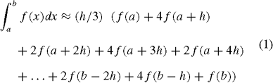
with error, assuming f ′′′′ exists on (a,b), given by

for some c in (a,b). The key features of the error term are the dependence on h4 and the f ′′′′ (c) term. These imply that doubling the number of subintervals (so that h is halved) yields approximately 1/16 the previous error (if the overall interval [a,b] is sufficiently small so that c does not vary too greatly), and the integral will be exact for polynomials of degree 3 or less, since f ′′′′ vanishes identically for such functions.

(Note that a method known as Richardson extrapolation can be used to improve Simpson's rule integral estimates even further if two different h values are used.)

As an example, the probability that a standard normal random variable has value between z = .5 and z = 1 is given by the integral of f(z) = exp(-z2/2)/√(2 π) from z = .5 to z = 1. Choosing n = 10, Simpson's rule estimates it to be (.05/3)(f (.5) + 4f (.55) + 2f (.6) + 4f (.65) + … + 4f (.95) + f(1)) or 0.14988228478…. Now f ′′′′(z) is (z4 – 6z2 + 3)f(z), and with c between .5 and 1, the error term is bounded from above by .6(.56)(.054)/180, that is, by 10–8. (The exact error is, in fact, 1.3 × 10–11.)

The logic underlying Simpson's rule considers f on m = n/2 equally spaced contiguous nonoverlapping subintervals, and on each subinterval of width 2h, it estimates the integral by using a quadratic interpolation. From the partition {a = x0, x1, …, b = x2m}, where xi+1 − xi = h, the integral of f on [x2j, x2j+2] for j = 0 to m − 1 is approximated by the integral of the quadratic function qj satisfying qj(x2j) = f(x2j), qj(x2j+1) = f(x2j+1), and qj(x2j+2) = f(x2j+2). By elementary calculus, the integral of qj on [x2j, x2j+2] is exactly (f(x2j) + 4f (x2j+1) + f (x2j+2))(h/3); it is more difficult to deduce that the error incurred on the subinterval is − f ′′′′ (c) h5/90 for some c in (x2j, x2j+2). Summing up estimates from all the subintervals yields Equation 1; collecting the errors and using the intermediate value property for derivatives gives the error term (Equation 2).

In its modern formulation, Simpson's rule is one of an infinite family of what are known as (closed-form) Newton-Cotes integration methods. (The trapezoid rule is another, less accurate, closed-form Newton-Cotes method; the midpoint rule is an open-form Newton-Cotes method.) Each estimates integrals by computing the exact integral of an appropriate (piece-wise) interpolating polynomial. Using any degree of interpolant, one can quickly deduce any Newton-Cotes weights, such as the h/3, 4h/3, h/3 for Simpson's rule, and so deduce ever more accurate integration schemes, as follows. Requiring that the integration method be exact for polynomials of degree d or lower and that the function be evaluated at equally spaced intervals leads quickly to linear conditions for the weights. For instance, in order to achieve exact integration results for polynomial integrands of degree through d = 2, consider the monomials f(x) = 1, x and x2 on the interval [0,2h]: Equating the integral with w0f (0) + w1f (1) + w2f (2) for these functions yields the system 2h = w0 + w1 + w2,2h2 = h w1 + 2h w2,8h3/3 = h2w1 + 4h2w2, whose solution is w0 = h/3 = w2, w1 = 4h/3. To determine the error term, assuming it has the form Kf(n)(c) (b − a)hk for some K, n, and k, apply the estimation to, for instance, f(x) = x4 on [0,2h]; since f ′′′′ (c) = 24 for any c, and the error[Page 896] incurred is −4h5/15, the error term must be − h4(b − a) f′′′′ (c)/180. Similarly, considering the related example of exact results for monomial integrands f(x) = 1,x,x2 and x3 on [0,3h], one obtains the weights w0 = 3h/8, w1 = 9h/8, w2 = 9h/8, w3 = 3h/8 (known as Simpson's “3/8” rule). Using f(x) = x4, the overall error term is found to be –h4(b − a) f ′′′′ (c)/80. (Note that the 3/8 rule, while based on a higher-degree interpolant than Simpson's rule, has a larger coefficient in its error term and ordinarily is not preferred to Simpson's rule. Its advantage is that it allows use of three subintervals. Thus, if data are supplied for an odd number of subintervals, the 3/8 rule can be used for the first three subintervals, and Simpson's rule can be applied to the others.)

...