Weibull Distribution

The Weibull distribution is named after the Swedish engineer Waloddi Weibull who used the distribution in a paper on the breaking strength of materials. As an example of Stigler's law of epynomy, Weibull was not the first to apply the distribution: Paul Rosen and Erich Rammler used it six years earlier to study the fineness of powdered coal. The distribution is used in areas as diverse as engineering (for reliability analysis), biostatistics (lifetime modeling and survival analysis), and psychology (for modeling response times).

The three-parameter Weibull cumulative distribution function (CDF) for a random variable T is defined as follows:

with θ > 0 and β > 0. The density function f(t) equals

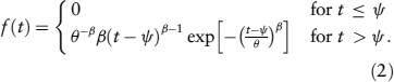
In the remainder of this entry, it is assumed that the distribution or density function can only be nonzero for t > Ψ, and this will not be written explicitly.

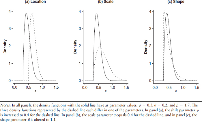
The three parameters Ψ, θ, and β of the Weibull distribution are the location, scale, and shape parameter, respectively. Changing Ψ results in a simple shift of the CDF and changing the scale parameter θ results in stretching or shrinking the CDF. The parameter β is a shape parameter because it affects the shape of the distribution (i.e., changing β affects more than just the location or the scale).

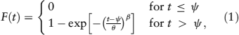
In Figure 1, the effects on the density function of changing each of these parameters in turn are shown. Parameter values are chosen in Figure 1 that result in densities that are realistic examples of common human response time densities. Weibull density functions are unimodal: For β ≤ 1, the mode of the Weibull density functions is located at Ψ but for β > 1, the single mode is larger than Ψ [and it is exactly at 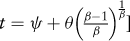. Most typically, the Weibull density functions exhibit right skew, but with an increasing β, it becomes more symmetric. If β becomes larger than 3.602, the density becomes left-skewed.

Sometimes it is more convenient to use a rate parameterization instead of the scale parameterization as in Equations 1 and 2. Applied to the CDF then gives:

with λ = θ–β (again, λ > 0). If the rate λ increases, the CDF becomes steeper and hence the density function will show less variability.

Properties

In this section, some properties of the Weibull distribution are investigated.

Mean, Variance, and Median

The mean of the Weibull distributed random variable T equals (using the location-scale parameterization):

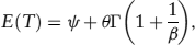
where Γ(x) is the gamma function. The variance of T is equal to

from which it can be seen that for a fixed value of Ψ, mean and variance are related. The median of the Weibull distribution is

[Page 1616]

Figure 1 Some Examples of the Weibull Density Functions with a Systematic Variation of the Parameters

All quantities can be expressed readily under the rate parameterization by replacing θ with .

Simulating Weibull Random Deviates

Simulating random draws from a Weibull distribution is easily done making use of the probability integral transform. In practice, one needs to draw a random number u, uniformly distributed between 0 and 1, and transform it as follows:

and t is then a draw from a Weibull distribution.

...