Entry
Reader's guide
Entries A-Z
Subject index
Decision Making Under Uncertainty
In decision making under uncertainty one studies how the single case (the decision maker, e.g., a radiologist) chooses between alternatives (e.g., presence or absence of a tumor on an X-ray) when the information presented is uncertain or incomplete. By evaluating two possible types of errors that the decision maker can make, false positives and false negatives, estimates of two independent characteristics of the decision maker are obtained. One characteristic is the decision maker's sensitivity, which is his or her ability to detect the presence of the “signal” (e.g., tumor). The second is the decision maker's response bias, which is his or her tendency to favor one of the possible alternatives (e.g., a higher willingness to err on the side of caution). In decision contexts where the two types of errors have differential payoffs or costs, or where the two alternatives are not equally likely to occur, the decision maker's decision process can be evaluated in more detail with the receiver operating characteristics (ROC) curve (also called the relative operating characteristics curve). Assessing these separate characteristics of the decision maker provides a more informative alternative to simply assessing his or her accuracy rate (e.g., overall percentage-correct decisions) and is one way of studying a single case, an individual, who is in the process of making a binary decision.
Conceptual Overview and Discussion
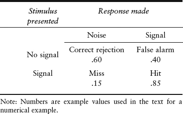
The simplest decision-making situation is when a decision maker must choose between two possible alternatives (e.g., disease or no disease). To assess the decision maker's sensitivity and response bias, the researcher uses two types of errors that the decision maker can make: a false alarm (false positive, or Type I error in statistical hypothesis testing) and a miss (false negative, or Type II error). Data for the estimates of these two probabilities are the relative frequencies of the decision maker's responses to each of the two alternative scenarios over repeated trials. Table 1 shows the possible situations that may arise. The stimulus presented to the decision maker is one of two, either containing a signal or not. The decision maker can make one of two responses, either signal present or not. This creates four possible outcomes, but note that because for a given stimulus the decision maker must give one of the two responses the probabilities within each row must add up to 1.0.
Table 1 Four possible outcomes in a two-choice decision task
Theoretical Basis: Signal Detection Theory
The theoretical basis for obtaining estimates of the decision maker's sensitivity and response bias is known as signal detection theory (SDT). SDT was developed and introduced into psychological research in the 1950s and is a direct application of statistical hypothesis testing to the tasks of detecting “signals” in noisy stimuli and of discriminating between two confusable stimuli. As in statistical hypothesis testing, there are two distributions, the noise-alone (analogous to the null) distribution and the signal + noise (alternative) distribution (see Figure 1). In SDT, the two distributions represent the probabilities of the various strength of evidence that the decision maker has for each of the two possible situations. The two distributions overlap, and there is one point, the decision criterion, along the evidence–strength axis that represents the decision maker's critical decision point for his or her decision rule. The rule applies on each trial and is stated thus: If the evidence received is stronger than the decision criterion, then respond “signal”; if the evidence is weaker, then respond “noise.” The evidence, however, can come from either of the two situations. So, if the strength of evidence falls above the criterion but was from the noise stimulus, fn distribution, then the decision maker has made an error of the false positive type (a false alarm). Alternatively, if it had in fact been from the signal distribution, fs, then the decision maker's response was correct and is referred to as a hit. The areas under the two curves to the right of the criterion are estimated by the proportions of P(hit) and P(false alarm) in Table 1.
...
- Case Study Research in Anthropology
- Case Study Research in Business and Management
- Case Study Research in Business Ethics
- Case Study Research in Education
- Case Study Research in Feminism
- Case Study Research in Medicine
- Case Study Research in Political Science
- Case Study Research in Psychology
- Case Study Research in Public Policy
- Case Study Research in Tourism
- Case Study With the Elderly
- Ecological Perspectives
- Healthcare Practice Guidelines
- Pedagogy and Case Study
- Before-and-After Case Study Design
- Blended Research Design
- Bounding the Case
- Case Selection
- Case-to-Case Synthesis
- Case Within a Case
- Comparative Case Study
- Critical Incident Case Study
- Cross-Sectional Design
- Decision Making Under Uncertainty
- Deductive-Nomological Model of Explanation
- Deviant Case Analysis
- Discursive Frame
- Dissertation Proposal
- Ethics
- Event-Driven Research
- Exemplary Case Design
- Extended Case Method
- Extreme Cases
- Healthcare Practice Guidelines
- Holistic Designs
- Hypothesis
- Integrating Independent Case Studies
- Juncture
- Longitudinal Research
- Mental Framework
- Mixed Methods in Case Study Research
- Most Different Systems Design
- Multimedia Case Studies
- Multiple-Case Designs
- Multi-Site Case Study
- Naturalistic Inquiry
- Natural Science Model
- Number of Cases
- Outcome-Driven Research
- Paradigmatic Cases
- Paradigm Plurality in Case Study Research
- Participatory Action Research
- Participatory Case Study
- Polar Types
- Problem Formulation
- Quantitative Single-Case Research Design
- Quasi-Experimental Design
- Quick Start to Case Study Research
- Random Assignment
- Research Framework
- Research Objectives
- Research Proposals
- Research Questions, Types of Retrospective Case Study
- Rhetoric in Research Reporting
- Sampling
- Socially Distributed Knowledge
- Spiral Case Study
- Statistics, Use of in Case Study
- Storyselling
- Temporal Bracketing
- Thematic Analysis
- Theory, Role of
- Theory-Testing With Cases
- Utilization
- Validity
- Agency
- Alienation
- Authenticity and Bad Faith
- Author Intentionality
- Case Study and Theoretical Science
- Contentious Issues in Case Study Research
- Cultural Sensitivity and Case Study
- Dissertation Proposal
- Ecological Perspectives
- Ideology
- Masculinity and Femininity
- Objectivism
- Othering
- Patriarchy
- Pluralism and Case Study
- Power
- Power/Knowledge
- Pragmatism
- Researcher as Research Tool
- Terroir
- Utilitarianism
- Verstehen
- Abduction
- Bayesian Inference and Boolean Logic
- Bricoleur
- Case-to-Case Synthesis
- Causal Case Study: Explanatory Theories
- Chronological Order
- Coding: Axial Coding
- Coding: Open Coding
- Coding: Selective Coding
- Cognitive Biases
- Cognitive Mapping
- Communicative Framing Analysis
- Complexity
- Computer-Based Analysis of Qualitative Data: ATLAS.ti
- Computer-Based Analysis of Qualitative Data: CAITA (Computer-Assisted Interpretive Textual Analysis)
- Computer-Based Analysis of Qualitative Data: Kwalitan
- Computer-Based Analysis of Qualitative Data: MAXQDA 2007
- Computer-Based Analysis of Qualitative Data: NVIVO
- Concept Mapping
- Congruence Analysis
- Constant Causal Effects Assumption
- Content Analysis
- Conversation Analysis
- Cross-Case Synthesis and Analysis
- Decision Making Under Uncertainty
- Document Analysis
- Factor Analysis
- Fiction Analysis
- High-Quality Analysis
- Inductivism
- Interactive Methodology, Feminist
- Interpreting Results
- Iterative
- Iterative Nodes
- Knowledge Production
- Method of Agreement
- Method of Difference
- Multicollinearity
- Multidimensional Scaling
- Over-Rapport
- Pattern Matching
- Re-Analysis of Previous Data
- Regulating Group Mind
- Relational Analysis
- Replication
- Re-Use of Qualitative Data
- Rival Explanations
- Secondary Data as Primary
- Serendipity Pattern
- Situational Analysis
- Standpoint Analysis
- Statistical Analysis
- Storyselling
- Temporal Bracketing
- Textual Analysis
- Thematic Analysis
- Use of Digital Data
- Utilization
- Webs of Significance
- Within-Case Analysis
- Action-Based Data Collection
- Analysis of Visual Data
- Anonymity and Confidentiality
- Anonymizing Data for Secondary Use
- Archival Records as Evidence
- Audiovisual Recording
- Autobiography
- Case Study Database
- Case Study Protocol
- Case Study Surveys
- Consent, Obtaining Participant
- Contextualization
- Critical Pedagogy and Digital Technology
- Cultural Sensitivity and Case Study
- Data Resources
- Depth of Data
- Diaries and Journals
- Direct Observation as Evidence
- Discourse Analysis
- Documentation as Evidence
- Ethnostatistics
- Fiction Analysis
- Field Notes
- Field Work
- Going Native
- Informant Bias
- Institutional Ethnography
- Interviews
- Iterative Nodes
- Language and Cultural Barriers
- Multiple Sources of Evidence
- Narrative Analysis
- Narratives
- Naturalistic Context
- Nonparticipant Observation
- Objectivity
- Over-Rapport
- Participant Observation
- Participatory Action Research
- Participatory Case Study
- Personality Tests
- Problem Formulation
- Questionnaires
- Reflexivity
- Regulating Group Mind
- Reliability
- Repeated Observations
- Researcher-Participant Relationship
- Re-Use of Qualitative Data
- Sensitizing Concepts
- Subjectivism
- Subject Rights
- Theoretical Saturation
- Triangulation
- Use of Digital Data
- Utilization
- Visual Research Methods
- Activity Theory
- Actor-Network Theory
- ANTi-History
- Autoethnography
- Base and Superstructure
- Case Study as a Methodological Approach
- Character
- Class Analysis
- Closure
- Codifying Social Practices
- Communicative Action
- Community of Practice
- Comparing the Case Study With Other Methodologies
- Consciousness Raising
- Contradiction
- Critical Discourse Analysis
- Critical Sensemaking
- Dasein
- Decentering Texts
- Deconstruction
- Dialogic Inquiry
- Discourse Ethics
- Double Hermeneutic
- Dramaturgy
- Ethnographic Memoir
- Ethnography
- Ethnomethodology
- Eurocentrism
- Families
- Formative Context
- Frame Analysis
- Front Stage and Back Stage
- Gendering
- Genealogy
- Governmentality
- Grounded Theory
- Hermeneutics
- Hybridity
- Imperialism
- Institutional Theory, Old and New
- Intertextuality
- Isomorphism
- Langue and Parôle
- Layered Nature of Texts
- Life History
- Logocentrism
- Management of Impressions
- Means of Production
- Metaphor
- Modes of Production
- Multimethod Research Program
- Multiple Selfing
- Native Points of View
- Negotiated Order
- Network Analysis
- One-Dimensional Culture
- Ordinary Troubles
- Organizational Culture
- Paradigm Plurality in Case Study Research
- Performativity
- Phenomenology
- Practice-Oriented Research
- Praxis
- Primitivism
- Qualitative Analysis in Case Study
- Qualitative Comparative Analysis
- Quantitative Single-Case Research Design
- Quick Start to Case Study Research
- Self-Confrontation Method
- Self-Presentation
- Sensemaking
- Sexuality
- Signifier and Signified
- Sign System
- Simulacrum
- Social-Interaction Theory
- Storytelling
- Structuration
- Symbolic Value
- Symbolic Violence
- Thick Description
- Writing and Difference
- Case Study and Theoretical Science
- Chicago School
- Colonialism
- Constructivism
- Critical Realism
- Critical Theory
- Dialectical Materialism
- Epistemology
- Existentialism
- Families
- Formative Context
- Frame Analysis
- Historical Materialism
- Interpretivism
- Liberal Feminism
- Managerialism
- Modernity
- North American Case Research Association
- Ontology
- Paradigm Plurality in Case Study Research
- Philosophy of Science
- Pluralism and Case Study
- Postcolonialism
- Postmodernism
- Postpositivism
- Poststructuralism
- Poststructuralist Feminism
- Radical Empiricism
- Radical Feminism
- Reality
- Scientific Method
- Scientific Realism
- Socialist Feminism
- Symbolic Interactionism
- Analytic Generalization
- Audience
- Authenticity
- Concatenated Theory
- Conceptual Argument
- Conceptual Model: Causal Model
- Conceptual Model: Operationalization
- Conceptual Model in a Qualitative Research Project
- Conceptual Model in a Quantitative Research Project
- Contribution, Theoretical
- Credibility
- Docile Bodies
- Equifinality
- Experience
- Explanation Building
- Extension of Theory
- Falsification
- Functionalism
- Generalizability
- Genericization
- Indeterminacy
- Indexicality
- Instrumental Case Study
- Macrolevel Social Mechanisms
- Middle-Range Theory
- Naturalistic Generalization
- Overdetermination
- Plausibility
- Probabilistic Explanation
- Process Tracing
- Program Evaluation and Case Study
- Reporting Case Study Research
- Rhetoric in Research Reporting
- Statistical Generalization
- Substantive Theory
- Theory-Building With Cases
- Theory-Testing With Cases
- Underdetermination
- ANTi-History
- Case Study as a Teaching Tool
- Case Study in Creativity Research
- Case Study Research in Tourism
- Case Study With the Elderly
- Collective Case Study
- Configurative-Ideographic Case Study
- Critical Pedagogy and Digital Technology
- Diagnostic Case Study Research
- Explanatory Case Study
- Exploratory Case Study
- Inductivism
- Institutional Ethnography
- Instrumental Case Study
- Intercultural Performance
- Intrinsic Case Study
- Limited-Depth Case Study
- Multimedia Case Studies
- Participatory Action Research
- Participatory Case Study
- Pluralism and Case Study
- Pracademics
- Processual Case Research
- Program Evaluation and Case Study
- Program-Logic Model
- Prospective Case Study
- Real-Time Cases
- Retrospective Case Study
- Re-Use of Qualitative Data
- Single-Case Designs
- Spiral Case Study
- Storyselling
- Loading...
Get a 30 day FREE TRIAL
-
 Watch videos from a variety of sources bringing classroom topics to life
 -
Read modern, diverse business cases
-
Explore hundreds of books and reference titles

Read next

More like this
Sage Recommends
We found other relevant content for you on other Sage platforms.
Have you created a personal profile? Login or create a profile so that you can save clips, playlists and searches